Bert-based NL2SQL Model: A Concise Baseline

Data Example

Each data sample is as follows:

{
    "table_id": "a1b2c3d4", # ID of the corresponding table
    "question": "The plot ratio of the new Shimao Maoyue Mansion project is greater than 1. What is its average area per unit?", # Natural language question
    "sql":{ # Ground truth SQL
        "sel": [7], # Columns selected by SQL 
        "agg": [0], # Aggregation functions for the selected columns, '0' means none
        "cond_conn_op": 0, # Relationship between conditions
        "conds": [
            [1, 2, "Shimao Maoyue Mansion"], # Condition column, condition type, condition value (col_1 == "Shimao Maoyue Mansion")
            [6, 0, "1"]
        ]
    }
}

# The condition operators, aggregation operators, and connection operators are as follows:
op_sql_dict = {0: ">", 1: "<", 2: "==", 3: "!="}
agg_sql_dict = {0: "", 1: "AVG", 2: "MAX", 3: "MIN", 4: "COUNT", 5: "SUM"}
conn_sql_dict = {0: "", 1: "and", 2: "or"}

Each sample corresponds to a data table containing all column names and corresponding data records. In principle, the generated SQL statements should be executable on the corresponding data table and return valid results.

As we can see, although it is called NL2SQL, the organizers have actually formatted the SQL statements very clearly. This way, the task can be significantly simplified. For example, the sel field is actually a multi-label classification model, except that the categories may change at any time because the categories here actually correspond to the columns of the data table. Since the data table and its meaning for each sample are different, we need to dynamically encode a category vector based on the column names of the table. As for agg, it corresponds one-to-one with sel and has fixed categories. cond_conn_op is a single-label classification problem.

The final conds is relatively more complex. It requires a combination of sequence labeling and classification because it must simultaneously determine which column is the condition, the operation relationship of the condition, and the value corresponding to the condition. It should be noted that the condition value is not always a fragment of the question; it might be a formatted result. For example, if the question says "year 16", the condition value might be the formatted "2016". However, since the organizers guarantee that the generated SQL can be executed in the corresponding data table and produce valid results, if the condition operator is "==", then the condition value will definitely appear in the values of the corresponding column in the data table. For instance, in the example sample above, the first column of the data table will definitely contain the value "Shimao Maoyue Mansion." We can use this information to calibrate the prediction results.

Model Structure

Before looking at this model, readers might want to think for themselves and consider how they would do it. Only after thinking will you understand where the difficulties lie, and only then can you understand the key points of some processing techniques in this model.

The schematic diagram of the model in this article is as follows:

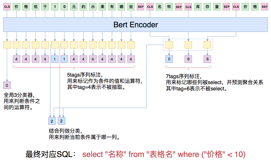
As a SQL query, the most basic requirement is to decide which columns will be selected. Since the meaning of the columns in each table is different, we concatenate the question sentence together with all the headers of the data table and input them into the Bert model for real-time encoding. Each header is also treated as a sentence, enclosed by [CLS]***[SEP]. After Bert, we obtain a series of encoding vectors, and then it depends on how we use these vectors.

The vector corresponding to the first [CLS] can be considered the sentence vector for the entire question. We use it to predict the connection operator for conds. The vectors corresponding to each subsequent [CLS] are considered encoding vectors for each table header. We extract them to predict whether the column represented by that header should be selected. Note that there is a trick in the prediction here: as mentioned earlier, besides predicting sel, we also need to predict the corresponding agg. There are 6 categories for agg, representing different operations. Given this, we simply add an extra category; the 7th category represents that this column is not selected. In this way, each column corresponds to a 7-class classification problem. If it falls into the first 6 classes, it means the column is selected and the agg is predicted simultaneously; if it falls into the 7th class, it means the column is not selected.

Now we are left with the more complex conds, such as where col_1 == value_1. col_1, value_1, and the operator == all need to be identified. The prediction of conds is divided into two steps: the first step predicts the condition value, and the second step predicts the condition column. Predicting the condition value is essentially a sequence labeling problem. Since there are 4 operators for the condition value, we similarly add one class to make it 5 classes. The 5th class represents that the current character is not labeled; otherwise, it is labeled. This allows us to predict the condition value and the operator. The remaining task is to predict the column corresponding to the condition value. We calculate the similarity between the character vectors of the labeled value and each header vector, and then apply softmax. My method for calculating similarity here is the simplest: directly concatenate the character vector and the header vector, pass them through a fully connected layer, and then a Dense(1). The reason for making it so simple is twofold: first, the main purpose of this article is to provide a basic feasible demo rather than a perfect program, leaving some room for improvement for readers; second, if it were made more complex, it would easily lead to OOM (Out of Memory) errors.

By the way, the model in this article was "created behind closed doors" based on the competition task. If readers wish to discuss mainstream NL2SQL models with me, I might be unable to help. Please understand.

Experimental Results

The model code for this article is located at:
https://github.com/bojone/bert_in_keras/blob/master/nl2sql_baseline.py

Note that if you encounter an error executing this code, you may need to modify Keras’s backend/tensorflow_backend.py. Change the line in the sparse_categorical_crossentropy function that was originally:

logits = tf.reshape(output, [-1, int(output_shape[-1])])

to:

logits = tf.reshape(output, [-1, tf.shape(output)[-1]])

I have already submitted this fix to the official repository, and it has been approved (see here). It should be automatically included in future versions.

Again, as long as you have carefully observed the competition data and thought independently about this task, the model introduced above is actually quite easy to understand. The fact that a simple model can achieve good results is due to Bert’s powerful semantic encoding capabilities. On the offline validation set, the SQL full match rate of the model in this article is about 58%. The official evaluation metric is (Full Match Rate + Execution Match Rate) / 2. This means you might write a SQL statement different from the annotated answer, but if the execution result is consistent, it counts as half correct.

Consequently, the final score will definitely be higher than 58%; I estimate it to be around 65%. Looking at the current leaderboard, 65% could place you in the top few (the top leader is currently at 70%). Since company employees are not allowed to participate in the leaderboard evaluation, I haven’t participated in the evaluation and don’t know what the online submission score would be. Interested contestants can submit and test for themselves.

By the way, it is best to have a 1080Ti or better graphics card to run this script. If you don’t have that much video memory, you can try reducing maxlen and batch size. Also, there are currently two available Chinese pre-trained weights for Bert: one is the official version, and the other is the Harbin Institute of Technology (HIT) version. The final results of both are similar, but the HIT version converges faster.

Looking at the entire model, the most difficult part of the implementation is carefully considering various masks. In the script mentioned above, xm, hm, cm are three mask variables used to remove the effects of the padding parts during the training process. Note that masking is not unique to Keras; whether you use Tensorflow or Pytorch, theoretically, you must handle masks carefully. If readers really cannot understand the mask part, feel free to leave a message for discussion. However, before asking, please answer the following questions:

What does the sequence look like before the mask? Which positions in the sequence changed after the mask? How did they change?

Answering this question proves that "you already understand what operations the program performed, you just don’t understand why it performed them that way." If you don’t even understand the operation itself, I think it will be difficult for us to communicate further (you should at least know which part changed...). It’s better to study Keras or Tensorflow properly before playing; you can’t expect to succeed in one step.

Pre- and Post-processing

For the model, the difficult part of implementation lies in the masks. However, if you look at the entire script, the parts that take up the most code are actually data reading, preprocessing, and result post-processing. The actual model construction only takes about twenty lines (marvel again at the conciseness of Keras and the power of Bert).

We mentioned that the condition value does not necessarily appear in the question. So how do we use the sequence labeling method on the question to extract the condition value?

My method is: if the condition value does not appear in the question, I segment the question and find all 1-grams, 2-grams, and 3-grams of the question. Then, I find the n-gram most similar to the condition value as the labeled fragment. During prediction, if an n-gram is found as a condition value and the operator is ==, we check if this n-gram has appeared in the database. If it has, we keep it directly; if not, we find the most similar value in the database.

The corresponding processes are reflected in the code; feel free to read it carefully.

Summary

Everyone is welcome to play 

https://tianchi.aliyun.com/markets/tianchi/zhuiyi_cn

Good luck to everyone!

When reposting, please include the original address: https://kexue.fm/archives/6771

For more detailed reposting matters, please refer to: "Scientific Space FAQ"