A Brief Introduction to VQ-VAE: Vector Quantized AutoEncoder

Interesting yet Mystifying

As an autoencoder, a distinct feature of VQ-VAE is that the encoded vectors are discrete. In other words, every element of the resulting encoding vector is an integer. This is the meaning of "Quantised," which we can also call "Quantization" (similar to "quanta" in quantum mechanics, implying discretization).

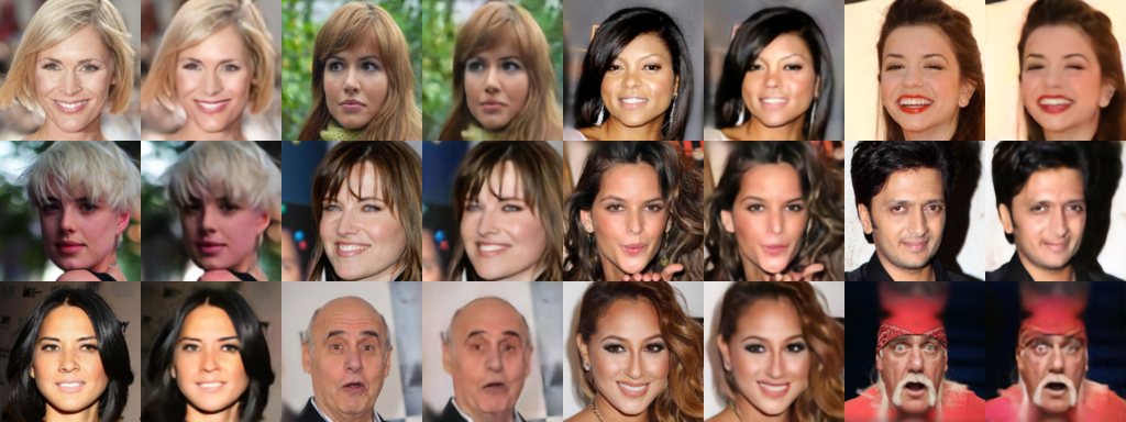
Even though the entire model is continuous and differentiable, the final encoding vectors are discrete, and the reconstruction results appear quite clear (as shown in the image at the beginning). This implies that VQ-VAE contains some interesting and valuable techniques worth learning. However, after reading the original paper, I felt it was somewhat difficult to understand—not because it was obscure like the ON-LSTM paper, but because it felt a bit "mystifying."

First, after reading the whole paper, you realize that VQ-VAE is actually an AE (AutoEncoder) rather than a VAE (Variational AutoEncoder). I don’t know why the authors insisted on using probabilistic language to associate it with VAE, which clearly increases the difficulty of understanding the paper. Second, one of the core steps of VQ-VAE is the Straight-Through Estimator, an optimization trick for discretizing latent variables. The original paper lacks a detailed explanation, making it necessary to look at the source code to understand what it means. Finally, the core philosophy of the paper isn’t well-articulated; it feels like it’s purely introducing the model itself without explaining the underlying ideas.

PixelCNN

To trace the origins of VQ-VAE’s ideas, one must discuss autoregressive models. It can be said that VQ-VAE’s approach to generative modeling stems from autoregressive models like PixelRNN and PixelCNN. These models recognize that the images we want to generate are actually discrete rather than continuous. Taking a CIFAR-10 image as an example, it is a 32 \times 32 3-channel image. In other words, it is a 32 \times 32 \times 3 matrix where each element is an integer from 0 to 255. Thus, we can view it as a sentence of length 32 \times 32 \times 3 = 3072 with a vocabulary size of 256. We can then use language modeling methods to generate an image pixel-by-pixel and recursively (predicting the next pixel given all previous pixels). This is the so-called autoregressive method: p(x)=p(x_1)p(x_2|x_1)\dots p(x_{3n^2}|x_1,x_2,\dots,x_{3n^2-1}) where each term p(x_1), p(x_2|x_1), \dots is a 256-way classification problem, albeit with different conditional dependencies.

There is plenty of information online about PixelRNN and PixelCNN, so I won’t repeat it here. I feel one could even ride the wave of BERT and create a "PixelAtt" (Attention) version. Research on autoregressive models mainly focuses on two aspects: one is how to design the recursion order to allow the model to better generate samples. Since image sequences are not simple 1D sequences (they are at least 2D, often 3D), whether you go "left-to-right then top-to-bottom," "top-to-bottom then left-to-right," or "center-to-outwards" significantly affects the generation quality. The other aspect is researching how to accelerate the sampling process. Among the literature I’ve read, a relatively new achievement in autoregressive models is the ICLR 2019 work "Generating High Fidelity Images with Subscale Pixel Networks and Multidimensional Upscaling".

The autoregressive approach is very stable and effective for probability estimation, but it has one fatal flaw: it is slow. Because it generates pixel-by-pixel, it requires random sampling for every single pixel. The CIFAR-10 example is considered a small image; convincing image generation today requires at least 128 \times 128 \times 3, which totals nearly 50,000 pixels. Generating a "sentence" of length 50,000 pixel-by-pixel is extremely time-consuming. Furthermore, for such long sequences, neither RNN nor CNN models can capture long-range dependencies effectively.

Original autoregressive models also have another issue: they sever the connection between categories. While it’s fine to treat each pixel as a 256-way classification problem because pixels are discrete, in reality, the difference between adjacent pixel values is very small. Pure classification problems fail to capture this relationship. More mathematically, our objective function, cross-entropy, is -\log p_t. If the target pixel is 100 and I predict 99, because the categories are different, p_t might be close to 0, making -\log p_t very large, resulting in a huge loss. But visually, there is little difference between a pixel value of 100 and 99; there shouldn’t be such a large penalty.

Dimensionality Reduction and Discretization

This solution seems natural and perhaps unremarkable, but in fact, it is not natural at all.

Since PixelCNN generates discrete sequences, if you want to model encoding vectors with PixelCNN, it means the encoding vectors must also be discrete. However, common dimensionality reduction methods, such as standard autoencoders, produce continuous encoding vectors that cannot directly generate discrete variables. Simultaneously, generating discrete variables often implies gradient vanishing problems. Furthermore, in the process of dimensionality reduction and reconstruction, how do we ensure the reconstructed image is not distorted? If the distortion is too severe—worse than a standard VAE—then VQ-VAE would have little value.

Fortunately, VQ-VAE provides an effective training strategy to solve these two problems.

Nearest Neighbor Reconstruction

In VQ-VAE, an n \times n \times 3 image x is first passed through an encoder to obtain a continuous encoding vector z: z = encoder(x) Here, z is a vector of size d. Additionally, VQ-VAE maintains an Embedding layer, which we can call a codebook, denoted as: E = [e_1, e_2, \dots, e_K] Each e_i is a vector of size d. Then, VQ-VAE maps z to one of these K vectors via nearest neighbor search: z \to e_k, \quad k = \mathop{\text{argmin}}_j \Vert z - e_j\Vert_2 We denote the codebook vector corresponding to z as z_q, and we consider z_q to be the final encoding result. Finally, z_q is passed to a decoder to reconstruct the original image \hat{x} = decoder(z_q).

The entire flow is: x \xrightarrow{encoder} z \xrightarrow{\text{Nearest Neighbor}} z_q \xrightarrow{decoder} \hat{x} In this way, because z_q is one of the vectors in the codebook E, it is effectively equivalent to one of the K integers 1, 2, \dots, K. Thus, this entire process is equivalent to encoding the entire image into a single integer.

Of course, the process described above is simplified. If we only encoded into a single vector, reconstruction would inevitably be distorted, and generalization would be hard to guarantee. Therefore, in practice, multiple convolutional layers are used to encode x into m \times m vectors of size d: z = \begin{pmatrix} z_{11} & z_{12} & \dots & z_{1m}\\ z_{21} & z_{22} & \dots & z_{2m}\\ \vdots & \vdots & \ddots & \vdots\\ z_{m1} & z_{m2} & \dots & z_{mm}\\ \end{pmatrix} That is, the total size of z is m \times m \times d. It still retains spatial structure. Each vector is then mapped to one in the codebook using the aforementioned method, resulting in a z_q of the same size, which is then used for reconstruction. Consequently, z_q is equivalent to an m \times m integer matrix, achieving discrete encoding.

Custom Gradients

We know that for a standard autoencoder, we can simply train using the following loss: \Vert x - decoder(z)\Vert_2^2 However, in VQ-VAE, we use z_q for reconstruction instead of z, so it seems we should use this loss: \Vert x - decoder(z_q)\Vert_2^2 But the problem is that the construction of z_q involves \text{argmin}, which is non-differentiable. If we use the second loss, we cannot update the encoder.

In other words, our goal is to minimize \Vert x - decoder(z_q)\Vert_2^2, but it is difficult to optimize. Meanwhile, \Vert x - decoder(z)\Vert_2^2 is easy to optimize but is not our actual target. What should we do? A crude method would be to use both: \Vert x - decoder(z)\Vert_2^2 + \Vert x - decoder(z_q)\Vert_2^2 But this isn’t ideal because minimizing \Vert x - decoder(z)\Vert_2^2 is not our goal and introduces extra constraints.

VQ-VAE uses a clever and direct method called the Straight-Through Estimator (STE). It originated from Bengio’s paper "Estimating or Propagating Gradients Through Stochastic Neurons for Conditional Computation". The VQ-VAE paper simply cites this without much explanation. In fact, reading the original paper is not very user-friendly; it’s better to look at the source code.

The idea of Straight-Through is simple: use the desired variable (even if non-differentiable) during forward propagation, and use a gradient you design yourself during backpropagation. Based on this idea, we design the objective function as: \Vert x - decoder(z + sg[z_q - z])\Vert_2^2 where sg stands for "stop gradient," meaning its gradient is not computed. Thus, during forward propagation (calculating loss), it is equivalent to decoder(z + z_q - z) = decoder(z_q). During backpropagation (calculating gradients), since z_q - z provides no gradient, it is equivalent to decoder(z), which allows us to optimize the encoder.

By the way, based on this idea, we can define custom gradients for many functions. For example, x + sg[\text{relu}(x) - x] defines the gradient of \text{relu}(x) as always being 1, while remaining equivalent to \text{relu}(x) during error calculation. Of course, we can use the same method to assign any gradient to a function; whether this has practical value depends on the specific task.

Maintaining the Codebook

Note that according to the nearest neighbor search design in VQ-VAE, we expect z_q and z to be very close (in fact, each vector in the codebook E appears as a cluster center for various z). However, this is not necessarily the case. Even if \Vert x - decoder(z)\Vert_2^2 and \Vert x - decoder(z_q)\Vert_2^2 are both small, it doesn’t mean z_q and z are close (i.e., f(z_1) = f(z_2) does not imply z_1 = z_2).

Therefore, to make z_q and z closer, we can directly add \Vert z - z_q\Vert_2^2 to the loss: \Vert x - decoder(z + sg[z_q - z])\Vert_2^2 + \beta \Vert z - z_q\Vert_2^2 Furthermore, we can be more precise. Since the codebook (z_q) is relatively free while z must ensure reconstruction quality, we should try to "make z_q move toward z" rather than "make z move toward z_q." Since the gradient of \Vert z_q - z\Vert_2^2 is the sum of the gradient with respect to z_q and the gradient with respect to z, we can decompose it into: \Vert sg[z] - z_q\Vert_2^2 + \Vert z - sg[z_q]\Vert_2^2 The first term fixes z and moves z_q toward z, while the second term fixes z_q and moves z toward z_q. Note that this "equivalence" applies to backpropagation (gradients); for forward propagation (loss), it is twice the original. Based on our discussion, we want z_q to move toward z more than z moves toward z_q, so we can adjust the final loss ratio: \Vert x - decoder(z + sg[z_q - z])\Vert_2^2 + \beta \Vert sg[z] - z_q\Vert_2^2 + \gamma \Vert z - sg[z_q]\Vert_2^2 where \gamma < \beta. In the original paper, \gamma = 0.25 \beta is used.

(Note: The codebook can also be updated using an exponential moving average; see the original paper for details.)

Fitting the Latent Distribution

After all this design, we have finally encoded the image into an m \times m integer matrix. Since this m \times m matrix preserves the spatial information of the original input image to some extent, we can use an autoregressive model like PixelCNN to fit the encoding matrix (i.e., model the prior distribution). Once we have the encoding distribution via PixelCNN, we can randomly generate a new encoding matrix, map it to a 3D real-valued matrix z_q (rows * columns * encoding dimension) via the codebook E, and finally pass it through the decoder to get an image.

Generally, the current m \times m is much smaller than the original n \times n \times 3. For example, in my experiments with the CelebA dataset, an original 128 \times 128 \times 3 image can be encoded into a 32 \times 32 matrix with almost no distortion. Thus, modeling the encoding matrix with an autoregressive model is much easier than modeling the original image directly.

Personal Reproduction

This is my implementation of VQ-VAE using Keras (Python 2.7 + Tensorflow 1.8 + Keras 2.2.4, with the model part referencing this repository):

https://github.com/bojone/vae/blob/master/vq_vae_keras.py

The main body of the script only contains the encoding and reconstruction of VQ-VAE (the image at the beginning of the article was reconstructed using this script, showing good results). It does not include the PixelCNN for modeling the prior. However, the comments at the end include an example of using Attention to model the prior distribution. After modeling the prior with Attention, the random sampling results are as follows:

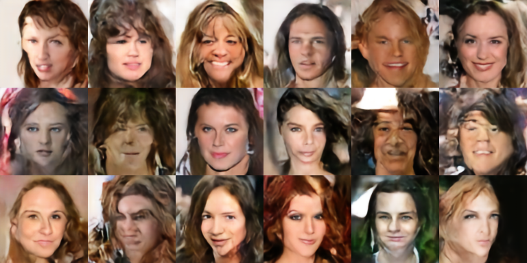
The results indicate that such random sampling is feasible, but the generation quality isn’t perfect. I used PixelAtt instead of PixelCNN because, in my reproduction, PixelCNN performed much worse than PixelAtt. Thus, PixelAtt has certain advantages, but its drawback is high VRAM usage, leading to OOM (Out Of Memory) errors. However, my personal reproduction being imperfect doesn’t mean the method itself is flawed; it could be due to tuning or the network not being deep enough. Personally, I am quite optimistic about research into discrete encoding.