A few days ago, several mathematics and physics groups were forwarding a problem posted by Teacher Li Yongle on his Weibo:
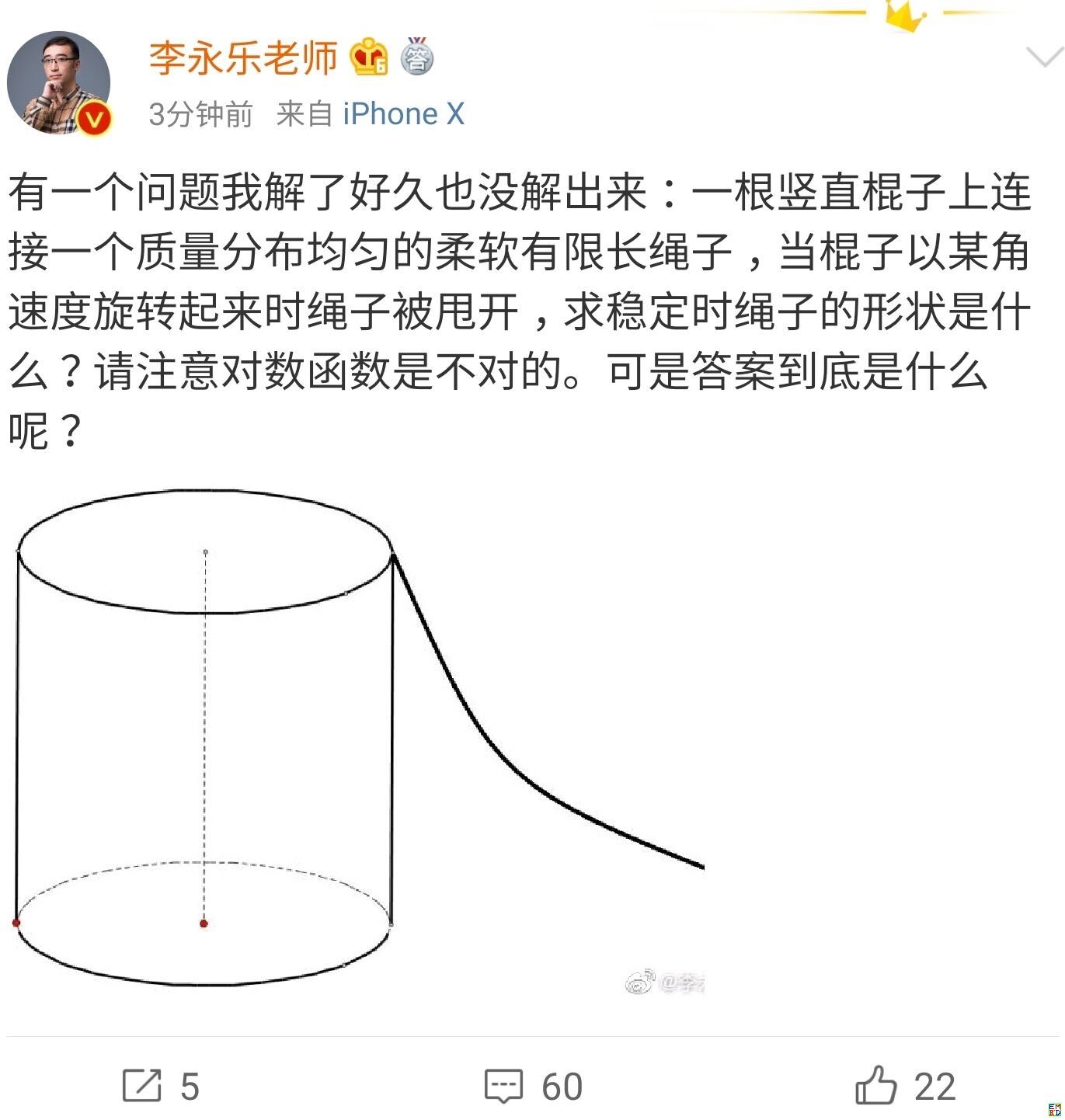
Realizing I hadn’t done any math or physics problems in a while, I gave it some thought and searched for some materials. I would like to share my findings with you here.
Related Content
In fact, the way Teacher Li Yongle presented it makes it feel like a pure physics exercise. However, this problem is actually related to the shapes of curves in many real-life examples. For instance, when you are jumping rope quickly (and the rope is taut), what is the shape of the rope?

The jump rope shape problem and the original problem proposed by Teacher Li Yongle are essentially equivalent. Their basic characteristics are:
There is a thin rope of uniform density;
The rope is spinning at a high speed, and the angular velocity \omega can be regarded as a constant;
The rope is also subject to gravity;
The goal is to find the curve shape when the rope reaches a (relative) static equilibrium.
Of course, in real life, air resistance also plays a role, which might mean the equilibrium state is not necessarily a planar curve. A typical example is the mosquito-repelling fans found on the market:

Derivation of the Equations
In this article, we are only concerned with the equilibrium formed in a plane. In this section, we will derive the corresponding differential equations. As an amateur physics enthusiast, I am not well-versed in professional force analysis. Instead, I will rely on the Principle of Least Action from the calculus of variations (refer to previous posts on this blog such as "Natural Extremum Series—8. Extremum Analysis", "Revisiting the ’Rotating Spring Extension’ Problem (Variational Solution)", "Corrections and Thoughts on the ’Equilibrium State Axiom’", and "A Brief Overview of Variations and Theoretical Mechanics").
The Principle of Least Action requires us to find the variation of the difference between kinetic energy and potential energy. For Teacher Li Yongle’s original problem, the rotational motion is horizontal, and gravity is vertical. Assuming the linear density is 1, the kinetic energy and potential energy are respectively: T = \int \frac{1}{2}\omega^2 x^2 \sqrt{dx^2+dy^2},\quad U = \int gy \sqrt{dx^2+dy^2} So, we are actually varying: S = \int \left(\frac{1}{2}\omega^2 x^2 - gy\right)\sqrt{dx^2+dy^2} = \int \left(\frac{1}{2}\omega^2 x^2 - gy\right) ds \label{eq:t}
In the case of jumping rope, both rotation and gravity are in the vertical direction (considering only the shape when the rope is at its lowest point). Thus, the target of variation is: S = \int \left(\frac{1}{2}\omega^2 y^2 - gy\right)ds This looks similar to [eq:t], but it is fundamentally different in terms of difficulty. By simply applying the transformation z = y - g/\omega^2, it becomes equivalent to the case of equation [eq:t] where g=0. As we will see later, this special case allows for an analytical solution, whereas the original equation [eq:t] does not.
The variational method is used when the two boundary points of the rope are fixed. However, in Teacher Li Yongle’s problem, it seems only one boundary point is fixed. Can we still use the variational method? In fact, we can. We can imagine that the other boundary point is also fixed (even if we don’t know its exact position); this does not change the original shape and trajectory.
Without further ado, let’s proceed with the variation. Let: \varphi(x, y) = \frac{1}{2}\omega^2 x^2 - gy We get: \begin{aligned} &\delta \int \varphi(x, y) ds \\ =& \int \left(\omega^2 x \delta x - g \delta y\right) ds + \varphi(x, y) \delta ds\\ =& \int \left(\omega^2 x \delta x - g \delta y\right) ds + \varphi(x, y) \frac{dx \delta dx + dy \delta dy}{ds}\\ =& \int \left(\omega^2 x \delta x - g \delta y\right) ds + \varphi(x, y) \left(\frac{dx}{ds}d\delta x + \frac{dy}{ds}d\delta y\right)\\ =& \int \left(\omega^2 x \delta x - g \delta y\right) ds - d\left(\varphi(x, y) \frac{dx}{ds}\right)\delta x - d\left(\varphi(x, y) \frac{dy}{ds}\right)\delta y \end{aligned} The last equality uses integration by parts and the convention that boundary conditions are zero, which are standard operations in the calculus of variations. Rearranging, we get: \begin{aligned} &\delta \int \varphi(x, y) ds \\ =& \int \left[\left(\omega^2 x - \frac{d}{ds}\left(\varphi(x, y) \frac{dx}{ds}\right)\right)\delta x + \left(-g - \frac{d}{ds}\left(\varphi(x, y) \frac{dy}{ds}\right)\right)\delta y\right]ds \end{aligned} Setting the terms for \delta x and \delta y to zero, we obtain the system of differential equations: \left\{\begin{aligned} &\frac{d}{ds}\left(\varphi(x, y) \frac{dx}{ds}\right)=\omega^2 x\\ &\frac{d}{ds}\left(\varphi(x, y) \frac{dy}{ds}\right) = -g \end{aligned}\right. Additionally, we have the condition: \left(\frac{dx}{ds}\right)^2 + \left(\frac{dy}{ds}\right)^2 = 1 \label{eq:ode1} From the second differential equation, we directly obtain: \varphi(x, y) \frac{dy}{ds} = -gs + C_1 \label{eq:ode2} Using [eq:ode1] and [eq:ode2], along with the boundary conditions, the shape of the curve can theoretically be solved.
Two Special Cases
At present, solving [eq:ode1] and [eq:ode2] analytically seems impossible. Therefore, we can analyze some special cases. The two simplest cases are \omega=0 or g=0.
\omega = 0
For \omega=0, in the context of Teacher Li Yongle’s problem, the answer is trivial: it is just a vertical line pointing downwards. However, we can add extra boundary conditions to make the result non-trivial—it becomes a "catenary." We have solved the catenary before (refer to "Natural Extremum Series—7. The Catenary Problem"). Let’s re-derive it here using [eq:ode1] and [eq:ode2]. When \omega=0, [eq:ode2] becomes: -gy\frac{dy}{ds} = -gs + C_1 Or equivalently: \frac{1}{2}\frac{d\left(y^2\right)}{ds} = s + C_1 (Letting the original -C_1/g be the new C_1), we solve to get: y^2 = s^2 + 2C_1 s + C_2 Without loss of generality, let C_1=0. Then (choosing an appropriate coordinate system so that C_2 is non-negative, we can denote C_2=a^2): s = \sqrt{y^2 - a^2}\quad \Rightarrow\quad ds = \frac{y dy}{\sqrt{y^2 - a^2}} Thus: \frac{\sqrt{dx^2 + dy^2}}{dy} = \frac{y}{\sqrt{y^2 - a^2}}\quad \Rightarrow\quad \frac{dx}{dy}=\frac{a}{\sqrt{y^2 - a^2}} Finally, we solve to get: x = a \cdot \text{arccosh}\left(\frac{y}{a}\right) + b\quad \Rightarrow\quad y = a\cosh \left(\frac{x - b}{a}\right) This is the catenary equation.
g = 0
As discussed earlier, when g=0, it corresponds to the shape of a jump rope. This is also called the "Rope skipping curve" or "Troposkien curve." In this case, [eq:ode2] becomes: \frac{1}{2}\omega^2 x^2 \frac{dy}{ds} = C_1\quad \Rightarrow\quad \frac{\sqrt{dx^2 + dy^2}}{dy} = \beta x^2 Which is: y=\int \frac{1}{\sqrt{\beta^2 x^4 - 1}}dx This involves elliptic integrals.
General Case
When neither \omega nor g is zero, the English search keywords are roughly "Shape of rotating rope / spinning lasso." This has been discussed on StackExchange. For those who can access Google, you can also look here.
While an analytical solution is not feasible, it does not prevent numerical solutions. For example:
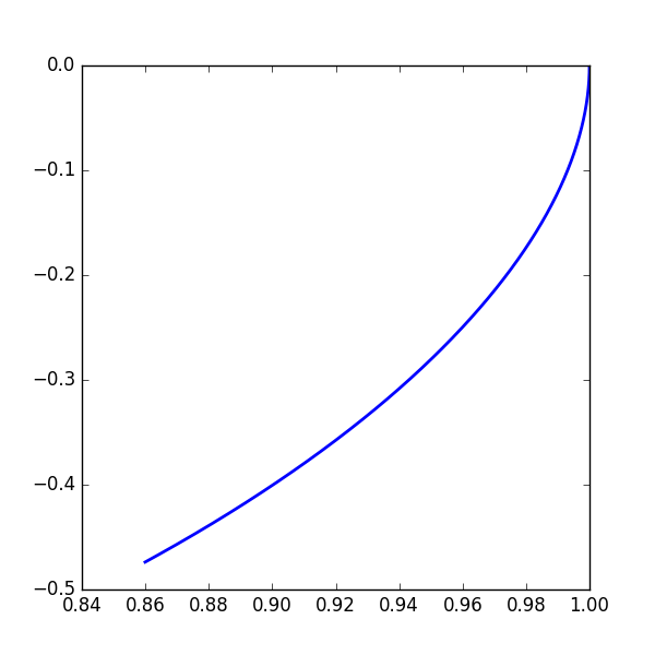
The reference code (Python) is as follows:
import numpy as np
from scipy.integrate import solve_ivp
import matplotlib.pyplot as plt

omega = 2
g = 3
T = 0.5
h = 0.0001
C1 = 0

def F(t, x):
    x, y = x
    G = (C1 - g * t) / (1 / 2. * omega**2 * x**2 - g * y)
    return [G, - np.sqrt(1 - G**2)]

x0, y0 = 1, 0.
ts = np.arange(0, T, h)
xs = solve_ivp(F, (0, T), [x0, y0], method='RK23', t_eval=ts)
x, y = xs.y
ts = xs.t

plt.clf()
plt.figure(figsize=(6, 6))
plt.plot(x, y, linewidth=2)
# plt.xlim(0.9, 1.15)
# plt.ylim(-0.25, 0)
plt.savefig('test.png')
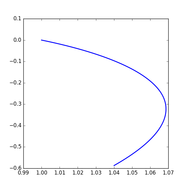
As mentioned before, the most general formulation of this problem involves two fixed endpoints. By adjusting C_1, we might obtain a curve like this (corresponding to C_1=1, a so-called "non-trivial solution"):
More related discussions can be found on Zhihu: https://www.zhihu.com/question/332446554/answer/746737923
Final Thoughts
Taking advantage of the popularity of Teacher Li Yongle’s problem, I took the opportunity to review some old physics knowledge and work through this problem. Of course, I couldn’t solve it completely in the general case, which ultimately required a return to numerical methods. However, the process of searching for information was quite rewarding.
I once had a dream of becoming a mathematician, physicist, or astronomer. Instead, I ended up doing odd jobs in the field of machine learning...
When reposting, please include the original article address: https://kexue.fm/archives/6784
For more detailed reposting matters, please refer to: "Scientific Space FAQ"