Optimization Algorithms from a Dynamics Perspective (III): A More Holistic View

The Direction of Steepest Descent

The basic explanation is this: the negative direction of the gradient is the direction in which the loss decreases fastest, so we use gradient descent. People usually draw a contour plot or similar diagram to explain why the negative gradient direction is the steepest descent direction. Consequently, many people criticize adaptive learning rate optimizers like RMSprop for a simple reason: they change the direction of parameter descent, making the optimization no longer follow the gradient direction, which supposedly leads to poor results.

But is this explanation reasonable enough?

Redefining the Problem

Before the formal discussion, let’s define the problem simply:

1. We have a scalar function L(\boldsymbol{\theta}) \geq 0, where the parameter \boldsymbol{\theta} can be a multi-dimensional vector.

2. There exists at least one point \boldsymbol{\theta}^* such that L(\boldsymbol{\theta}^*) = 0. That is, the minimum value of L(\boldsymbol{\theta}) is 0.

3. Given the specific form of L(\boldsymbol{\theta}), we naturally want to find \boldsymbol{\theta} such that L(\boldsymbol{\theta}) = 0. Even if that’s not possible, we want to find a \boldsymbol{\theta} that makes L(\boldsymbol{\theta}) as small as possible.

It is worth mentioning that point 2 is not strictly necessary, but it helps with the discussions we will explore later. In other words, point 2 is actually just an assumption. Generally, if we are given an arbitrary function to minimize, we don’t know its minimum value beforehand. However, in deep learning, this basically holds true because we usually set the loss to be non-negative, and thanks to the powerful fitting capabilities of neural networks, the loss can largely get close enough to 0.

Considering the Rate of Change of the Loss

Now, let’s get to the point. Suppose that during the optimization process, the parameter \boldsymbol{\theta} changes according to some trajectory \boldsymbol{\theta}(t). Then L(\boldsymbol{\theta}) also becomes a function of t, L(\boldsymbol{\theta}(t)). Note that t here is not real time; it is just a parameter used to describe the change, equivalent to the number of iterations.

Now we consider the rate of change of L(\boldsymbol{\theta}(t)): \frac{d}{dt}L(\boldsymbol{\theta}(t)) = \left\langle\nabla_{\boldsymbol{\theta}}L,\, \dot{\boldsymbol{\theta}}\right\rangle \label{eq:ld} Here \dot{\boldsymbol{\theta}} is d\boldsymbol{\theta}/dt, and \langle\cdot\rangle denotes the standard inner product. We want L to be as small as possible, so we naturally want the right side of the above equation to be negative, and its absolute value to be as large as possible. If we fix the magnitude of \dot{\boldsymbol{\theta}}, then to minimize the right side, according to the properties of the inner product, the angle between \nabla_{\boldsymbol{\theta}}L and \dot{\boldsymbol{\theta}} should be 180 degrees, which means: \dot{\boldsymbol{\theta}} = -\lambda \nabla_{\boldsymbol{\theta}}L \quad (\lambda > 0) \label{eq:gd} This explains that the negative gradient direction is indeed the direction of steepest descent. According to the first article, isn’t the above equation just gradient descent? Thus, we have derived gradient descent quite directly. Substituting [eq:gd] into [eq:ld], we get: \frac{d}{dt}L(\boldsymbol{\theta}(t)) = -\lambda \left\Vert\nabla_{\boldsymbol{\theta}}L\right\Vert^2 \label{eq:ld-1} This indicates that as long as the learning rate is small enough (simulating the ODE accurately enough) and \nabla_{\boldsymbol{\theta}}L \neq \boldsymbol{0}, then L will definitely decrease until \nabla_{\boldsymbol{\theta}}L = 0. At this point, the position is a local minimum or a saddle point; theoretically, it cannot be a local maximum. Furthermore, we often use Stochastic Gradient Descent (SGD). The mini-batch approach introduces a certain amount of noise, which to some extent can reduce the probability of staying at saddle points (as saddle points may not be robust to perturbations). Therefore, SGD usually performs better than full-batch gradient descent.

More Than One Direction

For example, although we have proved that the negative gradient direction is the steepest descent direction, why must we follow the steepest path? While the negative gradient is the "orthodox" path, one can also take unconventional routes. Theoretically, as long as I can guarantee a decrease, it’s fine. For instance, I could take: \dot{\boldsymbol{\theta}} = -\text{sign}\left(\nabla_{\boldsymbol{\theta}}L\right) \label{eq:rmsprop-1} Note that \nabla_{\boldsymbol{\theta}}L is a vector, and \text{sign}\left(\nabla_{\boldsymbol{\theta}}L\right) refers to taking the sign function of each component, resulting in a vector with elements -1, 0, or 1. Consequently, equation [eq:ld] becomes: \frac{d}{dt}L(\boldsymbol{\theta}(t)) = -\lambda \left\Vert\nabla_{\boldsymbol{\theta}}L\right\Vert_1 \label{eq:ld-2} where \Vert\boldsymbol{x}\Vert_1 = \sum_{i=1}^n |x_i| represents the L1 norm of the vector. This choice also guarantees that the loss decreases, and theoretically, it converges where \nabla_{\boldsymbol{\theta}}L = 0.

In fact, we also have (assuming non-zero gradient components): \text{sign}\left(\nabla_{\boldsymbol{\theta}}L\right) = \frac{\nabla_{\boldsymbol{\theta}}L}{\sqrt{\nabla_{\boldsymbol{\theta}}L \otimes \nabla_{\boldsymbol{\theta}}L}} \label{eq:rmsprop-2} Combining [eq:rmsprop-1] and the second article, and incorporating a moving average, we find that what we are discussing here is the RMSprop algorithm.

In other words, in adaptive learning rate optimizers, the fact that "the learning rate becomes a vector, making the optimization direction no longer the gradient direction" is not a flaw at all, and it should not be the reason adaptive learning rate optimizers are criticized.

What Happens if We Don’t Take the Shortcut?

However, the reality is that with fine-tuning, the final performance of adaptive learning rates is usually inferior to SGD, indicating that adaptive learning rate optimizers do have some issues. That is to say, if you take an unconventional path, although you might move faster than others initially, you might fall behind in the later stages.

Where is the problem? For Adagrad, the problem is obviously "stopping too early" because it sums the historical gradients (rather than averaging them), causing the learning rate to approach 0 too quickly in the later stages. For the RMSprop mentioned above, the problem is—"it simply won’t stop."

Combining [eq:rmsprop-1] and [eq:rmsprop-2], we get: \dot{\boldsymbol{\theta}} = -\frac{\nabla_{\boldsymbol{\theta}}L}{\sqrt{\nabla_{\boldsymbol{\theta}}L \otimes \nabla_{\boldsymbol{\theta}}L}} \label{eq:rmsprop-3} When does this algorithm stop? In fact, it won’t stop because as long as the gradient components are non-zero, the corresponding components of \frac{\nabla_{\boldsymbol{\theta}}L}{\sqrt{\nabla_{\boldsymbol{\theta}}L \otimes \nabla_{\boldsymbol{\theta}}L}} are also non-zero (either 1 or -1). Thus, from a theoretical standpoint, this algorithm has no fixed point, so it will never stop. To alleviate this, RMSprop in practice uses techniques like moving averages for the denominator and adding an epsilon (to prevent division by zero).

But this only alleviates the problem. In ODE terms, "this ODE is not asymptotically stable," so it will often miss the local optimum. This is the real problem with adaptive learning rate algorithms.

Guided by the Global Optimum

The starting point of this experiment is that whether it is [eq:gd] (with convergence rate [eq:ld-1]) or [eq:rmsprop-3] (with convergence rate [eq:ld-2]), even if they converge, they can only guarantee \nabla_{\boldsymbol{\theta}}L = 0, not that it is the global optimum (i.e., L(\boldsymbol{\theta}) = 0 is not guaranteed). So, a simple idea is: since we already know the minimum value is zero, why not incorporate this information?

Analogous to the previous reasoning, we can consider: \dot{\boldsymbol{\theta}} = -\frac{\nabla_{\boldsymbol{\theta}}L}{\left\Vert\nabla_{\boldsymbol{\theta}}L\right\Vert^2} L \label{eq:me-gd} In this case, equation [eq:ld] becomes very simple: \frac{d}{dt}L = -L This is just a simple linear differential equation, and its solution is L(t) = e^{-t}. As t \to +\infty, L(t) \to 0, which means the loss will definitely converge to zero.

Is It Really That Good?

Of course not. Let’s look at equation [eq:me-gd]. If we reach a local optimum where \nabla_{\boldsymbol{\theta}}L = \boldsymbol{0} but L > 0, then the right side of [eq:me-gd] becomes negative infinity. This is fine in theory, but impossible to implement in numerical calculations. Initially, I thought this problem was easy to solve—just add an epsilon to the denominator to avoid the origin. But further analysis revealed that this problem is fatal.

To see why, let’s rewrite [eq:me-gd] as: \dot{\boldsymbol{\theta}} = -\frac{\nabla_{\boldsymbol{\theta}}L}{\left\Vert\nabla_{\boldsymbol{\theta}}L\right\Vert} L \times \frac{1}{\left\Vert\nabla_{\boldsymbol{\theta}}L\right\Vert} \label{eq:me-gd-2} The problem is that 1/\left\Vert\nabla_{\boldsymbol{\theta}}L\right\Vert becomes infinite (a singularity). Can we use a truncation? For example, consider: \dot{\boldsymbol{\theta}} = -\frac{\nabla_{\boldsymbol{\theta}}L}{\left\Vert\nabla_{\boldsymbol{\theta}}L\right\Vert} L \times \min\left(\frac{1}{\left\Vert\nabla_{\boldsymbol{\theta}}L\right\Vert}, M\right) \label{eq:me-gd-3} where M \gg 0 is a constant, which bypasses the singularity. Doing this can indeed bypass some local optima, such as in the following example:

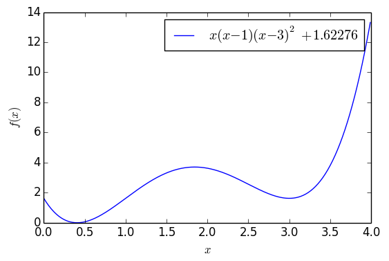
This function has a global optimum around x=0.41 where the function value is 0, but it has a secondary local optimum at x=3. If we start with x_0=4 and use pure gradient descent, it will basically converge to x=3. However, using [eq:me-gd-3] starting from x_0=4, after some oscillation, it can eventually converge to near x=0.41:

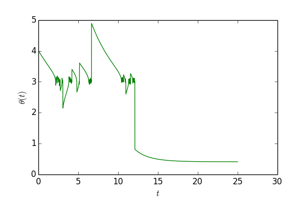
As we can see, it initially lingers near x=3, but after oscillating for a while, it jumps out and reaches the vicinity of x=0.41. The plotting code is as follows:

import numpy as np
import matplotlib.pyplot as plt

def f(x):
    return x * (x - 1) * (x - 3) * (x - 3) + 1.62276

def g(x):
    return -9 + 30 * x - 21 * x**2 + 4 * x**3

ts = [0]
xs = [4]
h = 0.01
H = 2500

for i in range(H):
    x = xs[-1]
    # delta = -sign(g(x)) * min(1/|g(x)|, 1000) * f(x)
    delta = -np.sign(g(x)) * min(abs(g(x)) / g(x)**2, 1000) * f(x)
    x += delta * h
    xs.append(x)
    ts.append(ts[-1] + h)

print(f(xs[-1]))
plt.figure()
plt.clf()
plt.plot(ts, xs, 'g')
plt.xlabel('$t$')
plt.ylabel('$\\theta(t)$')
plt.show()

However, while it looks beautiful, it actually has little value because to guarantee jumping out of all local optima, M must be large enough (to be close enough to the original [eq:me-gd-2]), and the number of iterations must be sufficient. But if these conditions are met, it’s actually better to just add Gaussian noise to gradient descent. As shown in the first article, if we assume the gradient noise is Gaussian, then from a probabilistic standpoint, it can always reach the global optimum (given enough iterations). Therefore, this seemingly elegant thing doesn’t have much practical value.

(Note: I later learned that Polyak had studied the form of the learning rate in [eq:me-gd] long ago. Searching for "Polyak step size" will yield many related works, such as "Revisiting the Polyak step size" and "Generalized Polyak Step Size for First Order Optimization with Momentum".)