Weight Decay and Learning Rate from the Perspective of Moving Average

Moving Average

The general form of Weight Decay is: \begin{equation} \boldsymbol{\theta}_t = \boldsymbol{\theta}_{t-1} - \eta_t (\boldsymbol{u}_t + \lambda_t \boldsymbol{\theta}_{t-1}) \end{equation} where \boldsymbol{\theta} represents the parameters, \boldsymbol{u} is the update amount provided by the optimizer, and \lambda_t, \eta_t are what we call Weight Decay and Learning Rate, respectively. The entire sequences \{\lambda_t\} and \{\eta_t\} are referred to as the "WD Schedule" and "LR Schedule." Introducing the notation: \begin{equation} \begin{aligned} \boldsymbol{m}_t =&\, \beta_1 \boldsymbol{m}_{t-1} + \left(1 - \beta_1\right) \boldsymbol{g}_t, & \hat{\boldsymbol{m}}_t =&\, \boldsymbol{m}_t\left/\left(1 - \beta_1^t\right)\right. &\\ \boldsymbol{v}_t =&\, \beta_2 \boldsymbol{v}_{t-1} + \left(1 - \beta_2\right) \boldsymbol{g}_t^2,& \hat{\boldsymbol{v}}_t =&\, \boldsymbol{v}_t\left/\left(1 - \beta_2^t\right)\right. & \end{aligned} \end{equation} Then, for SGDM, we have \boldsymbol{u}_t=\boldsymbol{m}_t; for RMSProp, \boldsymbol{u}_t= \boldsymbol{g}_t/(\sqrt{\boldsymbol{v}_t} + \epsilon); for Adam, \boldsymbol{u}_t=\hat{\boldsymbol{m}}_t\left/\left(\sqrt{\hat{\boldsymbol{v}}_t} + \epsilon\right)\right.; for SignSGDM, \boldsymbol{u}_t=\mathop{\text{sign}}(\boldsymbol{m}_t); and for Muon, \boldsymbol{u}_t=\mathop{\text{msign}}(\boldsymbol{m}_t). Except for SGDM, the examples listed here are all considered types of adaptive learning rate optimizers.

Our starting point is the Exponential Moving Average (EMA) perspective, rewriting Weight Decay as: \begin{equation} \boldsymbol{\theta}_t = (1 - \lambda_t \eta_t)\boldsymbol{\theta}_{t-1} - \eta_t \boldsymbol{u}_t = (1 - \lambda_t \eta_t)\boldsymbol{\theta}_{t-1} + \lambda_t \eta_t ( -\boldsymbol{u}_t / \lambda_t)\label{eq:wd-ema} \end{equation} In this form, Weight Decay appears as a weighted average of the model parameters and -\boldsymbol{u}_t / \lambda_t. The moving average perspective is not new; articles such as "How to set AdamW’s weight decay as you scale model and dataset size" and "Power Lines: Scaling Laws for Weight Decay and Batch Size in LLM Pre-training" have discussed it. This article aims to calculate various aspects more carefully within this perspective.

The following sections primarily use Adam as an example, followed by a discussion on the applicability to other optimizers. The calculation process overlaps significantly with "Asymptotic Estimation of Weight RMS in AdamW (Part 1)" and "Asymptotic Estimation of Weight RMS in AdamW (Part 2)"; readers may refer to them for comparison.

Iterative Expansion

For simplicity, let us first consider constant \lambda, \eta. Let \beta_3 = 1 - \lambda\eta, then \boldsymbol{\theta}_t = \beta_3 \boldsymbol{\theta}_{t-1} + (1 - \beta_3)( -\boldsymbol{u}_t / \lambda). This is formally consistent with \boldsymbol{m}_t and \boldsymbol{v}_t. Expanding the iteration directly gives: \begin{equation} \boldsymbol{\theta}_t = \beta_3^t \boldsymbol{\theta}_0 + (1 - \beta_3)\sum_{i=1}^t \beta_3^{t-i} (-\boldsymbol{u}_i / \lambda) \end{equation} For Adam, \boldsymbol{u}_t=\hat{\boldsymbol{m}}_t\left/\left(\sqrt{\hat{\boldsymbol{v}}_t} + \epsilon\right)\right.. Generally, at the end of training, t is large enough such that \beta_1^t, \beta_2^t are sufficiently close to zero, so we do not need to distinguish between \boldsymbol{m}_t and \hat{\boldsymbol{m}}_t, or \boldsymbol{v}_t and \hat{\boldsymbol{v}}_t. Furthermore, simply setting \epsilon=0, we can simplify to \boldsymbol{u}_t=\boldsymbol{m}_t / \sqrt{\boldsymbol{v}_t}. Applying a classic mean-field approximation: \begin{equation} \underbrace{\frac{1-\beta_3}{1-\beta_3^t}\sum_{i=1}^t \beta_3^{t-i} \boldsymbol{u}_i}_{\text{denoted as } \bar{\boldsymbol{u}}_t} = \frac{1-\beta_3}{1-\beta_3^t}\sum_{i=1}^t \beta_3^{t-i} \frac{\boldsymbol{m}_i}{\sqrt{\boldsymbol{v}_i}}\approx \frac{\bar{\boldsymbol{m}}_t \,\,\triangleq\,\, \frac{1-\beta_3}{1-\beta_3^t}\sum_{i=1}^t \beta_3^{t-i}\boldsymbol{m}_i}{\sqrt{\bar{\boldsymbol{v}}_t \,\,\triangleq\,\, \frac{1-\beta_3}{1-\beta_3^t}\sum_{i=1}^t \beta_3^{t-i}\boldsymbol{v}_i}}\label{eq:u-bar} \end{equation} Expanding \boldsymbol{m}_t and \boldsymbol{v}_t gives \boldsymbol{m}_t = (1 - \beta_1)\sum_{i=1}^t \beta_1^{t-i}\boldsymbol{g}_i and \boldsymbol{v}_t = (1 - \beta_2)\sum_{i=1}^t \beta_2^{t-i}\boldsymbol{g}_i^2. Substituting these into the above: \begin{gather} \bar{\boldsymbol{m}}_t = \frac{(1-\beta_3)(1 - \beta_1)}{1-\beta_3^t}\sum_{i=1}^t \beta_3^{t-i} \sum_{j=1}^i \beta_1^{i-j}\boldsymbol{g}_j = \frac{(1-\beta_3)(1 - \beta_1)}{(1-\beta_3^t)(\beta_3 - \beta_1)}\sum_{j=1}^t (\beta_3^{t-j+1} - \beta_1^{t-j+1})\boldsymbol{g}_j\\[6pt] \bar{\boldsymbol{v}}_t = \frac{(1-\beta_3)(1 - \beta_2)}{1-\beta_3^t}\sum_{i=1}^t \beta_3^{t-i} \sum_{j=1}^i \beta_2^{i-j}\boldsymbol{g}_j^2 = \frac{(1-\beta_3)(1 - \beta_2)}{(1-\beta_3^t)(\beta_3 - \beta_2)}\sum_{j=1}^t (\beta_3^{t-j+1} - \beta_2^{t-j+1})\boldsymbol{g}_j^2 \end{gather} The exchange of summation symbols is based on the identity \sum_{i=1}^t \sum_{j=1}^i a_i b_j = \sum_{j=1}^t \sum_{i=j}^t a_i b_j. In summary, we have: \begin{equation} \boldsymbol{\theta}_t = \beta_3^t \boldsymbol{\theta}_0 + (1 - \beta_3^t)(-\bar{\boldsymbol{u}}_t / \lambda) \label{eq:theta-0-bar-u} \end{equation} The weight \boldsymbol{\theta}_t is our desired training result, expressed as a weighted average of \boldsymbol{\theta}_0 and -\bar{\boldsymbol{u}}_t / \lambda. Here, \boldsymbol{\theta}_0 is the initial weight, and \bar{\boldsymbol{u}}_t is data-dependent. Under the mean-field approximation, it is approximately \bar{\boldsymbol{m}}_t/\sqrt{\bar{\boldsymbol{v}}_t}, where \bar{\boldsymbol{m}}_t and \bar{\boldsymbol{v}}_t can be expressed as a weighted sum of gradients at each step. Taking \bar{\boldsymbol{m}}_t as an example, the weight of the gradient at step j is proportional to \beta_3^{t-j+1} - \beta_1^{t-j+1}.

Memory Cycle

We are primarily concerned with pre-training, which is characterized by being Single-Epoch; most data is only seen once. Therefore, one of the keys to achieving good results is not to forget early data. Assuming the training data has been globally shuffled, it is reasonable to consider the data in each batch to be equally important.

Data is linearly superimposed into \bar{\boldsymbol{m}}_t in the form of gradients. Assuming each step’s gradient only contains information from the current batch, then for a certain batch not to be forgotten, the coefficient \beta_3^{t-j+1} - \beta_1^{t-j+1} cannot be too small. Examining the function f(s) = \beta_3^s - \beta_1^s, it is a function that first increases and then decreases. However, because \beta_3 is closer to 1 than \beta_1, the increasing phase is short, and it mostly follows an exponential decay at larger distances, as shown below:

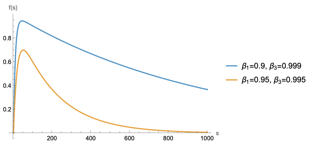
In short, the trend is that the further the distance, the smaller the coefficient. To prevent the model from forgetting any batch, the coefficient at the furthest point cannot be too small. Assuming the coefficient must be no less than c \in (0, 1) to be remembered, when s is large enough, \beta_1^s tends to 0 first, so \beta_3^s - \beta_1^s \approx \beta_3^s. Solving \beta_3^s \geq c yields s \leq \frac{\log c}{\log \beta_3} \approx \frac{-\log c}{\lambda\eta}. This indicates that the model can remember at most \mathcal{O}(1/\lambda\eta) steps of data, which is its memory cycle.

Would setting \lambda=0 to make the memory cycle infinite solve the forgetting problem? Theoretically, yes, but it is not a good choice. Weight Decay also serves to help the model forget its initialization. From Equation [eq:theta-0-bar-u], the weight of the initialization \boldsymbol{\theta}_0 is \beta_3^t. If \beta_3 is too large or the number of training steps t is too small, the proportion of initialization remains high, and the model may still be in an underfitting stage.

Furthermore, Weight Decay helps stabilize the model’s "internal dynamics" (or "internal medicine"). In "Asymptotic Estimation of Weight RMS in AdamW (Part 1)", we derived that the asymptotic Weight RMS of AdamW is \sqrt{\eta/2\lambda}. If \lambda=0, the Weight RMS will expand at a rate of \eta\sqrt{t}. This means that setting \lambda=0 directly might lead to weight explosion and other internal model abnormalities.

Therefore, \beta_3 cannot be too small to avoid forgetting early data, nor can it be too large to avoid underfitting or weight explosion. A suitable setting is to make 1/\lambda\eta proportional to the number of training steps. In a Multi-Epoch training scenario, one might consider making 1/\lambda\eta proportional to the number of training steps in a single epoch.

Dynamic Version

In actual training, we more commonly use dynamic LR Schedules, such as Cosine Decay, Linear Decay, or WSD (Warmup-Stable-Decay). Thus, the results for static Weight Decay and Learning Rate do not fully align with practice, and we need to generalize them to a dynamic version.

Starting from Equation [eq:wd-ema], using the approximation 1 - \lambda_t \eta_t \approx e^{-\lambda_t \eta_t} and expanding the iteration, we get: \begin{equation} \boldsymbol{\theta}_t = (1 - \lambda_t \eta_t)\boldsymbol{\theta}_{t-1} - \eta_t \boldsymbol{u}_t \approx e^{-\lambda_t \eta_t}\boldsymbol{\theta}_{t-1} - \eta_t \boldsymbol{u}_t = e^{-\kappa_t}\left(\boldsymbol{\theta}_0 - \sum_{i=1}^t e^{\kappa_i}\eta_i\boldsymbol{u}_i\right) \end{equation} where \kappa_t = \sum_{i=1}^t \eta_i\lambda_i. Letting z_t = \sum_{i=1}^t e^{\kappa_i}\eta_i, we obtain the same mean-field approximation: \begin{equation} \bar{\boldsymbol{u}}_t\triangleq\frac{1}{z_t}\sum_{i=1}^t e^{\kappa_i}\eta_i \boldsymbol{u}_i = \frac{1}{z_t}\sum_{i=1}^t e^{\kappa_i}\eta_i \frac{\boldsymbol{m}_i}{\sqrt{\boldsymbol{v}_i}}\approx \frac{\bar{\boldsymbol{m}}_t \,\,\triangleq\,\, \frac{1}{z_t}\sum_{i=1}^t e^{\kappa_i}\eta_i\boldsymbol{m}_i}{\sqrt{\bar{\boldsymbol{v}}_t \,\,\triangleq\,\, \frac{1}{z_t}\sum_{i=1}^t e^{\kappa_i}\eta_i\boldsymbol{v}_i}} \end{equation} Substituting the expansions for \boldsymbol{m}_t and \boldsymbol{v}_t: \begin{gather} \bar{\boldsymbol{m}}_t = \frac{1}{z_t}\sum_{i=1}^t e^{\kappa_i}\eta_i\boldsymbol{m}_i = \frac{1 - \beta_1}{z_t}\sum_{i=1}^t e^{\kappa_i}\eta_i\sum_{j=1}^i \beta_1^{i-j}\boldsymbol{g}_j = \sum_{j=1}^t\boldsymbol{g}_j\underbrace{\frac{1 - \beta_1}{z_t}\sum_{i=j}^t e^{\kappa_i}\beta_1^{i-j}\eta_i}_{\text{denoted as }\bar{\beta}_1(j,t)} \\ \bar{\boldsymbol{v}}_t = \frac{1}{z_t}\sum_{i=1}^t e^{\kappa_i}\eta_i\boldsymbol{v}_i = \frac{1 - \beta_2}{z_t}\sum_{i=1}^t e^{\kappa_i}\eta_i\sum_{j=1}^i \beta_2^{i-j}\boldsymbol{g}_j^2 = \sum_{j=1}^t\boldsymbol{g}_j^2\underbrace{\frac{1 - \beta_2}{z_t}\sum_{i=j}^t e^{\kappa_i}\beta_2^{i-j}\eta_i}_{\text{denoted as }\bar{\beta}_2(j,t)} \\ \end{gather} As we can see, compared to the static case, the dynamic version does not change much in form, except that the gradient weighting coefficients become the slightly more complex \bar{\beta}_1(j,t) and \bar{\beta}_2(j,t). Specifically, when \beta_1, \beta_2 \to 0, \bar{\beta}_1(j,t) and \bar{\beta}_2(j,t) simplify to: \begin{equation} \bar{\beta}_1(j,t) = \bar{\beta}_2(j,t) = \frac{e^{\kappa_j}\eta_j}{z_t}\label{eq:bb1-bb2-0} \end{equation}

Optimal Schedule

There are many things we can do next, the most basic being calculating \bar{\beta}_1(j,t) and \bar{\beta}_2(j,t) or estimating the memory cycle based on specific WD and LR Schedules. However, here we choose to do something more extreme—directly deriving an optimal WD and LR Schedule.

Specifically, we previously assumed that the data is globally shuffled, so each batch is equally important. However, the coefficient \bar{\beta}_1(j,t) \propto \beta_3^{t-j+1} - \beta_1^{t-j+1} obtained in the static version is not a constant but varies with distance, which does not perfectly align with the idea that "every batch is equally important." Ideally, we would want it to be constant. Based on this expectation, we can solve for the corresponding \lambda_j, \eta_j.

For simplicity, we start with the special case \beta_1, \beta_2 \to 0. We want to solve the equation e^{\kappa_j}\eta_j/z_t = c_t, where c_t is a function depending only on t. Note that the "constant" mentioned above is with respect to j; since t is the end of training, the constant can depend on it. To simplify the solution, we use integration instead of summation, i.e., \kappa_s \approx \int_0^s \lambda_{\tau} \eta_{\tau} d\tau. The equation becomes \exp\left(\int_0^s \lambda_{\tau} \eta_{\tau} d\tau\right)\eta_s \approx c_t z_t. Taking the logarithm of both sides and differentiating with respect to s: \begin{equation} \lambda_s \eta_s + \frac{\dot{\eta}_s}{\eta_s} \approx 0 \label{eq:lr-wd-ode} \end{equation} If \lambda_s is a constant \lambda, we can solve for: \begin{equation} \eta_s \approx \frac{\eta_{\max}}{\lambda\eta_{\max} s + 1}\label{eq:opt-lrt-wd} \end{equation} This is the optimal LR Schedule under constant Weight Decay. It does not require a preset endpoint t or a minimum learning rate \eta_{\min}, meaning it can continue training indefinitely, similar to the Stable phase of WSD, but it automatically balances the coefficients of each gradient step. However, it has a drawback: as s \to \infty, it tends to 0. From "Asymptotic Estimation of Weight RMS in AdamW (Part 2)", we know that Weight RMS tends toward \lim\limits_{s\to\infty} \frac{\eta_s}{2\lambda_s}, so this drawback might pose a risk of weight collapse.

To solve this, we can consider letting \lambda_s = \alpha\eta_s, where \alpha=\lambda_{\max}/\eta_{\max} is a constant. In this case, we solve for: \begin{equation} \eta_s \approx \frac{\eta_{\max}}{\sqrt{2\lambda_{\max}\eta_{\max} s + 1}},\qquad \lambda_s \approx \frac{\lambda_{\max}}{\sqrt{2\lambda_{\max}\eta_{\max} s + 1}} \label{eq:opt-lrt-wdt} \end{equation} Correspondingly, e^{\kappa_s} \approx \sqrt{2\lambda_{\max}\eta_{\max} s + 1}, e^{\kappa_s}\eta_s \approx \eta_{\max}, z_t \approx \eta_{\max} t, and \bar{\beta}_1(j,t) = \bar{\beta}_2(j,t) \approx 1/t.

General Results

The current results, such as Equation [eq:opt-lrt-wd] and Equation [eq:opt-lrt-wdt], are based on \beta_1, \beta_2 = 0. Do the results need to change when they are non-zero? More generally, to what extent can these results, which are based on the Adam optimizer, be generalized to other optimizers?

First, regarding the case where \beta_1, \beta_2 \neq 0: the answer is that when t is large enough, the conclusion does not need major modification. Taking \bar{\beta}_1(j,t) as an example, under the optimal schedule described above, e^{\kappa_i}\eta_i is a constant (related to t). According to the definition: \begin{equation} \bar{\beta}_1(j,t) = \frac{1 - \beta_1}{z_t}\sum_{i=j}^t e^{\kappa_i}\beta_1^{i-j}\eta_i \propto \sum_{i=j}^t \beta_1^{i-j} = \frac{1 - \beta_1^{t-j+1}}{1 - \beta_1} \end{equation} When t is large enough, \beta_1^{t-j+1} \to 0, so this can also be seen as a constant independent of j. As mentioned earlier, for \beta_1, \beta_2, the condition that "t is large enough" is almost certainly satisfied, so we can directly use the results for \beta_1, \beta_2 = 0.

As for the optimizers, we mentioned SGDM, RMSProp, Adam, SignSGDM, and Muon. These can be divided into two categories. SGDM is one category; its \bar{\boldsymbol{u}}_t is directly \bar{\boldsymbol{m}}_t, so even the mean-field approximation is unnecessary. Thus, results up to Equation [eq:lr-wd-ode] are applicable. However, Equation [eq:opt-lrt-wd] and Equation [eq:opt-lrt-wdt] are likely not the most suitable, because the asymptotic Weight RMS of SGDM also depends on the gradient norm [Reference], so the gradient norm must be taken into account, making it relatively more complex.

The remaining RMSProp, Adam, SignSGDM, and Muon fall into the other category: adaptive learning rate optimizers. Their update rules all have a homogeneous form of \frac{\text{gradient}}{\sqrt{\text{gradient}^2}}. In this case, if we still believe in the mean-field approximation, we get the same \bar{\boldsymbol{m}}_t and the same \beta_1(j,t), so the results up to Equation [eq:lr-wd-ode] are applicable. Furthermore, for this class of homogeneous optimizers, it can be proven that Weight RMS is also asymptotically proportional to \sqrt{\eta/\lambda}, so Equation [eq:opt-lrt-wd] and Equation [eq:opt-lrt-wdt] can also be reused.

Discussion of Hypotheses

Our derivation has reached a temporary conclusion. In this section, let’s discuss the hypotheses upon which the derivation relies.

Throughout the text, there are two major hypotheses worth discussing. The first is the mean-field approximation, first introduced in "Rethinking Learning Rate and Batch Size (Part 2): Mean Field". Mean field itself is certainly not new—it is a classic approximation in physics—but its use to analyze optimizer dynamics was likely first introduced by the author. It has been used to estimate the optimizer’s Batch Size, Update RMS, and Weight RMS, and the results appear reasonable.

Regarding the validity of the mean-field approximation, we cannot say too much; it reflects a kind of faith. On one hand, based on the reasonableness of existing estimation results, we believe it will continue to be reasonable, at least for providing effective asymptotic estimates for some scalar indicators. On the other hand, for adaptive learning rate optimizers, the non-linearity of their update rules greatly increases the difficulty of analysis. Besides the mean-field approximation, we actually have few other calculation tools to use.

The most typical example is Muon. Because it is a non-element-wise operation, previous component-wise calculation methods like those for SignSGD lose their effectiveness, while the mean-field approximation still works (refer to "Rethinking Learning Rate and Batch Size (Part 3): Muon"). Therefore, the mean-field approximation actually provides a unified, effective, and concise calculation method for analyzing and estimating a large class of adaptive learning rate optimizers. Currently, no other method seems to have the same effect, so we must continue to trust it.

The second major hypothesis is that "each step’s gradient only contains information from the current batch." This hypothesis is essentially incorrect because the gradient depends not only on the current batch’s data but also on the parameters from the previous step, which naturally contain historical information. However, we can try to remedy this: theoretically, every batch brings new information; otherwise, the batch would have no reason to exist. So the remedy is to change it to "each step’s gradient contains roughly the same amount of incremental information."

Of course, upon closer reflection, this statement is also controversial because the more one learns and the wider the coverage, the less unique information subsequent batches contain. However, we can still struggle a bit by dividing knowledge into two categories: "patterns" and "facts." Factual knowledge—for example, that a certain theorem was discovered by a certain mathematician—can only be learned by heart. Thus, we could change it to "each step’s gradient contains roughly the same amount of factual knowledge." In any case, from a practical standpoint, an LR Schedule derived from "treating every gradient step equally" seems to have benefits, so one can always try to construct an explanation for it.

A recent paper, "How Learning Rate Decay Wastes Your Best Data in Curriculum-Based LLM Pretraining", provides indirect evidence. It considers curriculum learning where data quality increases over time and finds that aggressive LR Decay makes the advantages of curriculum learning disappear. Our result is that the weight of each batch is given by Equation [eq:bb1-bb2-0], which is proportional to the Learning Rate. If the LR Decay is too aggressive, the weight of later high-quality data becomes too small, leading to poor results. Being able to reasonably explain this phenomenon conversely demonstrates the reasonableness of our hypothesis.

Summary

This article understands Weight Decay (WD) and Learning Rate (LR) from the perspective of moving averages and explores the optimal WD Schedule and LR Schedule from this perspective.

Reprinting: Please include the original link: https://kexue.fm/archives/11459

Further details on reprinting: Please refer to "Scientific Space FAQ".