To this day, LDM (Latent Diffusion Models) remains the mainstream paradigm for diffusion models. By using an Encoder to highly compress the original images, LDM significantly reduces the computational costs of training and inference while also lowering the difficulty of training, achieving multiple benefits at once. However, high compression also implies information loss, and the "compression, generation, decompression" pipeline lacks some of the beauty of end-to-end systems. Consequently, there has always been a group of researchers dedicated to "returning to pixel space," hoping to let diffusion models complete generation directly on the original data.
The paper to be introduced in this article, "Back to Basics: Let Denoising Generative Models Denoise", follows this line of thought. Based on the fact that original data often resides on a low-dimensional sub-manifold, it proposes that models should predict the data rather than the noise. This leads to "JiT (Just image Transformers)," which significantly simplifies the architecture of pixel-space diffusion models.
Signal-to-Noise Ratio
Undoubtedly, the "main force" of today’s diffusion models is still LDM. Even the recently discussed RAE only claims that LDM’s Encoder is "outdated" and suggests replacing it with a new, stronger Encoder, but it does not change the "compress then generate" pattern.
The reason for this situation, besides LDM’s ability to significantly reduce the cost of generating large images, is a key observation researchers made over a long period: directly performing high-resolution diffusion generation in pixel space seemed to face "inherent difficulties." Specifically, when configurations that worked well at low resolutions (such as Noise Schedules) were applied to high-resolution diffusion model training, the results were significantly worse, manifesting as slow convergence and FIDs inferior to low-resolution models.
Later, works like Simple Diffusion realized the key reason for this phenomenon: when the same Noise Schedule is applied to higher-resolution images, the signal-to-noise ratio (SNR) essentially increases. Specifically, if we apply noise of the same intensity to a small image and a large image and then scale them to the same size, the large image will appear clearer. Therefore, using the same Noise Schedule to train high-resolution diffusion models unintentionally makes the denoising task easier, leading to issues like low training efficiency and poor performance.
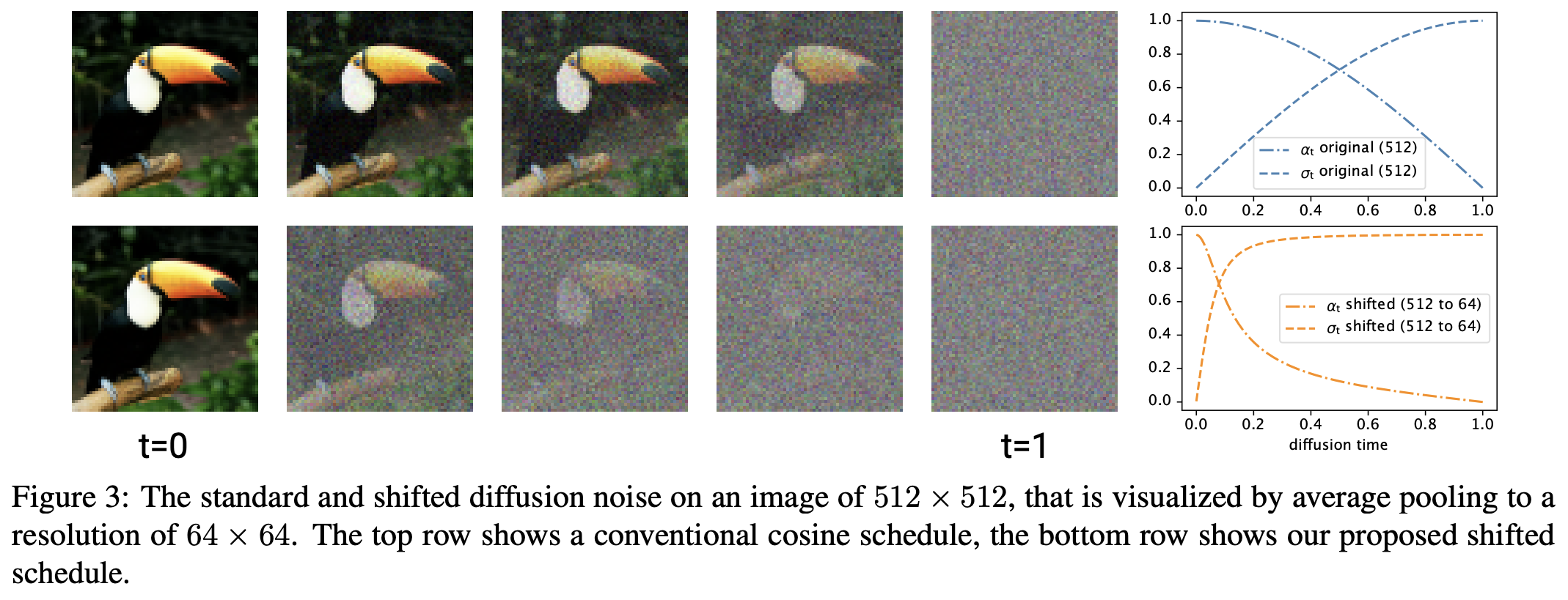
Once this reason was understood, the solution was not hard to find: adjust the Noise Schedule of the high-resolution diffusion model by increasing the corresponding noise intensity to align the SNR at each step. For a more detailed discussion, one can refer to the previous blog post "Generative Diffusion Models (22): SNR and Large Image Generation (Part 1)". Since then, diffusion models in pixel space have gradually caught up with LDM’s performance and begun to demonstrate their own competitiveness.
Model Bottleneck
However, although pixel-space diffusion models have caught up with LDM in terms of metrics (such as FID or IS), another puzzling problem remains: to achieve metrics similar to low-resolution models, high-resolution models must pay more in terms of computation, such as more training steps, larger models, or larger feature maps.
Some readers might think this is fine: generating larger images requires more cost, which seems reasonable. At first glance, this makes sense, but upon closer inspection, it is not entirely scientific. Generating large images might be inherently more difficult, but at least for metrics like FID/IS, it shouldn’t be, because these two metrics are calculated after scaling the generated results to a specific size. This means if we have a set of small images, obtaining a set of large images with the same FID/IS is easy—just upsample each small image, which has almost zero extra cost.
At this point, someone might point out that "upsampled large images lack detail." True, that is the "inherent difficulty" mentioned earlier—generating more detail. However, the upsampling operation is at least invariant for FID and IS. This implies that, theoretically, if I invest the same amount of computational power, I should at least be able to obtain a large image generation model with roughly the same FID/IS, even if the details are insufficient. But the reality is not so; often, we only get a model that is significantly worse in all aspects.
Let’s concretize this problem. Suppose the baseline is a 128 \times 128 small image model that
patchifies the input into 8 \times 8
patches, linearly projects them to 768 dimensions, feeds them into a ViT
with hidden_size=768, and finally projects them back to the
image size. This configuration works well at 128 \times 128 resolution. Now, for 512 \times 512 large image generation, I only
need to change the patch size to 32 \times
32. Aside from the input/output projections becoming slightly
larger, the overall computational volume remains almost unchanged.
The question is: using such a model with roughly the same computational cost to train a 512 \times 512 diffusion model, can we get the same FID/IS as the 128 \times 128 resolution model?
Low-Dimensional Manifold
For diffusion models before JiT, the answer is likely no, because such models have a low-rank bottleneck at high resolutions.
Previously, there were two mainstream paradigms for diffusion models: one is predicting noise like DDPM, and the other is predicting the difference between noise and the original image (velocity) like ReFlow. Both regression targets involve noise. Noise vectors are sampled independently and identically from a normal distribution; they "fill" the entire space. In mathematical terms, their support is the entire space. Consequently, for a model to successfully predict arbitrary noise vectors, it must not have a low-rank bottleneck; otherwise, it cannot even implement an identity mapping, let alone denoising.
Returning to the previous example, when the patch size is changed to 32 \times 32, the input dimension is 32 \times 32 \times 3 = 3072, which is then projected down to 768 dimensions. This is naturally irreversible. Therefore, if we still use it to predict noise or velocity, it will perform poorly due to the low-rank bottleneck. The key issue here is that actual models do not truly have universal fitting capabilities but rather possess various fitting bottlenecks.
At this point, the core modification of JiT is ready to be revealed:
Compared to noise, the effective dimension of original data is often much lower. That is to say, original data resides in a lower-dimensional sub-manifold. This means that predicting data is "easier" for the model than predicting noise. Therefore, the model should prioritize predicting the original data, especially when network capacity is limited.
Simply put, original data like images often have specific structures, making them easier to predict. Thus, the model should predict the image, which minimizes the impact of the low-rank bottleneck and might even turn a disadvantage into an advantage.
Individually, none of these points are new: that noise support is the full space and that original data resides on a low-dimensional manifold are conclusions that are "widely known" to some extent. As for directly using the model to predict images instead of noise, this is not the first attempt either. But the most remarkable part of the original paper is connecting these points together to form a reasonable explanation that is both surprising and hard to refute, feeling almost like "it should have been this way all along."
Experimental Analysis
Of course, while it sounds reasonable, so far it is at most a hypothesis. Next comes the experimental validation. There are many experiments in JiT, but the author believes the following three are most noteworthy.
First, we now have three optional prediction targets: noise, velocity, and data. These can be further divided into the model’s prediction target and the loss function’s regression target, resulting in 9 combinations. Taking ReFlow as an example, let \boldsymbol{x}_0 be noise and \boldsymbol{x}_1 be data. Its training objective is: \mathbb{E}_{\boldsymbol{x}_0\sim p_0(\boldsymbol{x}_0),\boldsymbol{x}_1\sim p_1(\boldsymbol{x}_1)}\bigg[\bigg\Vert \boldsymbol{v}_{\boldsymbol{\theta}}\big(\underbrace{(\boldsymbol{x}_1 - \boldsymbol{x}_0)t + \boldsymbol{x}_0}_{\boldsymbol{x}_t}, t\big) - (\boldsymbol{x}_1 - \boldsymbol{x}_0)\bigg\Vert^2\bigg] where \boldsymbol{v}=\boldsymbol{x}_1 - \boldsymbol{x}_0 is the velocity. This is a loss where the regression target is velocity (\boldsymbol{v}\text{-loss}). If we use a neural network to model \boldsymbol{v}_{\boldsymbol{\theta}}(\boldsymbol{x}_t, t), then the model’s prediction target is also velocity (\boldsymbol{v}\text{-pred}). If we use \boldsymbol{x}_1 - \boldsymbol{x}_0=\frac{\boldsymbol{x}_1 - \boldsymbol{x}_t}{1-t} to parameterize \boldsymbol{v}_{\boldsymbol{\theta}}(\boldsymbol{x}_t, t) as \frac{\text{NN}_{\boldsymbol{\theta}}(\boldsymbol{x}_t, t) - \boldsymbol{x}_t}{1-t}, then the prediction target of the \text{NN} is the data \boldsymbol{x}_1 (\boldsymbol{x}\text{-pred}).
The performance of these 9 combinations on ViT models with and without low-rank bottlenecks is shown in the figure below (left):
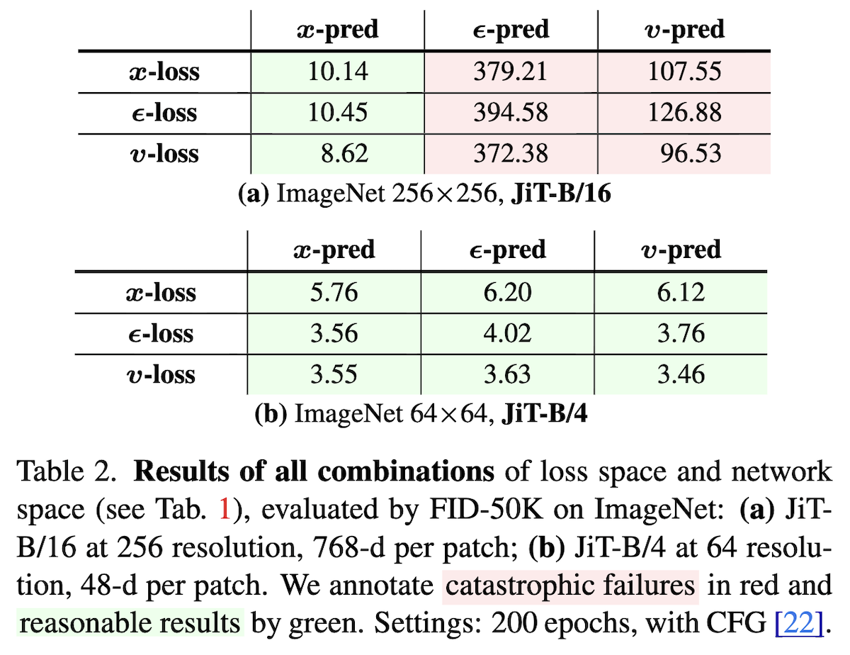
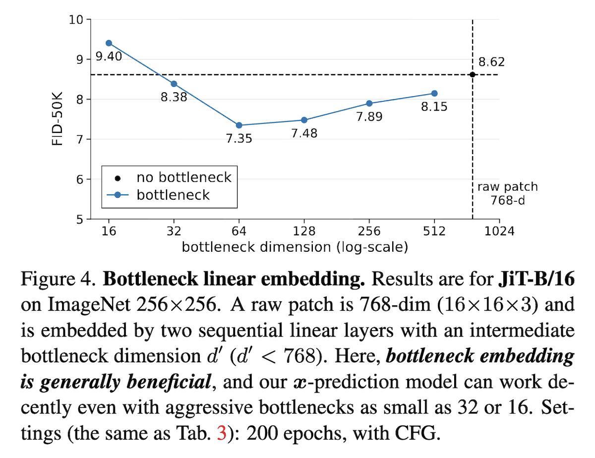
As can be seen, if there is no low-rank bottleneck (b), the 9 combinations do not differ much. However, if the model has a low-rank bottleneck (a), only when the prediction target is data (\boldsymbol{x}\text{-pred}) can training succeed. The impact of the regression target is relatively secondary, confirming the necessity of predicting data. Furthermore, the paper found that actively adding an appropriate low-rank bottleneck to the \boldsymbol{x}\text{-pred} JiT actually benefits FID, as shown in the figure above (right).
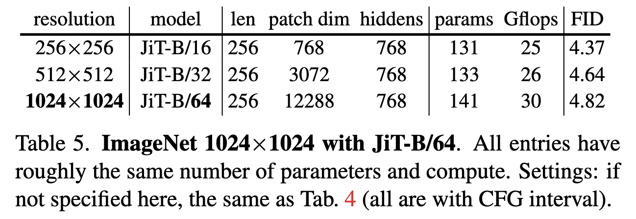
Further, the table below verifies that by predicting data, it is indeed possible to obtain models of different resolutions with similar FID under similar computational and parameter costs:
Finally, the author also conducted a comparison, using a ViT model with large patch sizes on CelebA HQ to compare the effects of \boldsymbol{x}\text{-pred} and \boldsymbol{v}\text{-pred} (trained roughly, for comparison only):
Extended Thinking
For more experimental results, please refer to the original paper. In this section, let’s discuss what changes JiT brings to diffusion models.
First, it does not refresh the SOTA. From the experimental tables in the paper, for the task of generating ImageNet images, it does not bring a new SOTA, though the gap with the best results is small. Thus, its performance can be considered SOTA-level, but it hasn’t significantly surpassed existing ones. On the other hand, changing an existing SOTA non-\boldsymbol{x}\text{-pred} model to \boldsymbol{x}\text{-pred} likely won’t yield significantly better results.
However, it might reduce the cost of achieving SOTA. Letting the model predict data alleviates the impact of low-rank bottlenecks, allowing us to re-examine lightweight designs that were previously discarded due to poor performance, or to "upgrade" low-resolution SOTA models to high resolution with low additional training costs. From this perspective, the real problem JiT solves is transferability from low resolution to high resolution.
Additionally, JiT makes the architectures for visual understanding and generation more unified. In fact, JiT is essentially the same ViT model used for visual understanding, and it differs little from the GPT architecture of text LLMs. Architectural unification is more conducive to designing multimodal models that integrate understanding and generation. In contrast, the standard architecture for previous diffusion models was U-Net, which contains multi-level up/downsampling and multiple cross-scale skip connections, making the structure relatively complex.
From this viewpoint, JiT accurately identifies the most critical skip connection in U-Net. Returning to the ReFlow example, if we understand it as modeling \boldsymbol{v}_{\boldsymbol{\theta}}(\boldsymbol{x}_t, t), then in JiT we have \boldsymbol{v}_{\boldsymbol{\theta}}(\boldsymbol{x}_t, t)=\frac{\text{NN}_{\boldsymbol{\theta}}(\boldsymbol{x}_t, t) - \boldsymbol{x}_t}{1-t}. The extra -\boldsymbol{x}_t is precisely a skip connection from input to output. U-Net, on the other hand, doesn’t care which connection is critical; it simply adds such a skip connection to every up/downsampling block.
Finally, a "side note." JiT reminds the author of DDCM, which requires pre-sampling a huge "T \times \text{img\_size}" matrix as a codebook. The author once tried to simulate it using a linear combination of a finite number of random vectors but failed. This experience made the author deeply realize that i.i.d. noise fills the entire space and is incompressible. Therefore, when seeing JiT’s viewpoint that "data resides on a low-dimensional manifold and predicting data is easier than predicting noise," the author understood and accepted it almost instantly.
Summary
This article briefly introduced JiT. Based on the fact that original data often resides on a low-dimensional sub-manifold, it proposes that models should prioritize predicting data rather than noise or velocity. This reduces the modeling difficulty of diffusion models and decreases the likelihood of negative outcomes like model collapse.
Original address: https://kexue.fm/archives/11428
For more details on reprinting, please refer to: "Scientific Space FAQ"