Descriptions like "the opposite direction of the gradient is the direction of steepest descent" are frequently used to introduce the principles of Stochastic Gradient Descent (SGD). However, this statement is conditional. For instance, "direction" is mathematically defined as a unit vector, which depends on the definition of a "norm (magnitude)." Different norms lead to different conclusions. For example, Muon actually replaces the norm for matrix parameters with the spectral norm, thereby obtaining a new descent direction. Furthermore, when we move from unconstrained optimization to constrained optimization, the direction of steepest descent is not necessarily the opposite direction of the gradient.
To this end, in this article, we will start a new series using "constraints" as the main thread to re-examine the proposition of "steepest descent" and explore where the "direction of steepest descent" points under different conditions.
Optimization Principle
As the first article, we will start from SGD to understand the mathematical meaning behind the phrase "the opposite direction of the gradient is the direction of steepest descent," and then apply it to optimization on a hypersphere. Before that, however, I would like to revisit the Least Action Principle for optimizers mentioned in "Muon Sequel: Why Did We Choose to Try Muon?".
This principle attempts to answer "what makes a good optimizer." First, we certainly hope the model converges as quickly as possible. However, due to the complexity of neural networks, if the steps taken are too large, the training is likely to collapse. Therefore, a good optimizer should be both stable and fast—ideally, it should significantly reduce the loss without requiring major changes to the model. Mathematically, this can be written as: \min_{\Delta \boldsymbol{w}} \mathcal{L}(\boldsymbol{w} +\Delta\boldsymbol{w}) \qquad \text{s.t.}\qquad \rho(\Delta\boldsymbol{w})\leq \eta where \mathcal{L} is the loss function, \boldsymbol{w}\in\mathbb{R}^n is the parameter vector, \Delta \boldsymbol{w} is the update amount, and \rho(\Delta\boldsymbol{w}) is some measure of the size of the update \Delta\boldsymbol{w}. The above objective is intuitive: find the update that reduces the loss function the most (fast) under the premise that the "step" does not exceed \eta (stable). This is the mathematical meaning of the "Least Action Principle" and also the mathematical meaning of "steepest descent."
Target Transformation
Assuming \eta is small enough, \Delta\boldsymbol{w} will also be small enough such that a first-order approximation is sufficiently accurate. We can then replace \mathcal{L}(\boldsymbol{w} +\Delta\boldsymbol{w}) with \mathcal{L}(\boldsymbol{w}) + \langle\boldsymbol{g},\Delta\boldsymbol{w}\rangle, where \boldsymbol{g} = \nabla_{\boldsymbol{w}}\mathcal{L}(\boldsymbol{w}), obtaining the equivalent objective: \min_{\Delta \boldsymbol{w}} \langle\boldsymbol{g},\Delta\boldsymbol{w}\rangle \qquad \text{s.t.}\qquad \rho(\Delta\boldsymbol{w})\leq \eta This simplifies the optimization objective into a linear function of \Delta \boldsymbol{w}, reducing the difficulty of solving it. Furthermore, let \Delta \boldsymbol{w} = -\kappa \boldsymbol{\varphi}, where \rho(\boldsymbol{\varphi})=1. Then the above objective is equivalent to: \max_{\kappa,\boldsymbol{\varphi}} \kappa\langle\boldsymbol{g},\boldsymbol{\varphi}\rangle \qquad \text{s.t.}\qquad \rho(\boldsymbol{\varphi}) = 1, \,\,\kappa\in[0, \eta] Assuming we can find at least one \boldsymbol{\varphi} satisfying the condition such that \langle\boldsymbol{g},\boldsymbol{\varphi}\rangle\geq 0, then \max\limits_{\kappa\in[0,\eta]} \kappa\langle\boldsymbol{g},\boldsymbol{\varphi}\rangle = \eta\langle\boldsymbol{g},\boldsymbol{\varphi}\rangle. That is, the optimization of \kappa can be solved beforehand, resulting in \kappa=\eta. The final equivalent problem leaves only the optimization of \boldsymbol{\varphi}: \max_{\boldsymbol{\varphi}} \langle\boldsymbol{g},\boldsymbol{\varphi}\rangle \qquad \text{s.t.}\qquad \rho(\boldsymbol{\varphi}) = 1 \label{eq:core} Here, \boldsymbol{\varphi} satisfies the condition that some "magnitude" \rho(\boldsymbol{\varphi}) equals 1, so it represents the definition of a "direction vector." Maximizing its inner product with the gradient \boldsymbol{g} means finding the direction that makes the loss decrease the fastest (i.e., the opposite direction of \boldsymbol{\varphi}).
Gradient Descent
From Equation [eq:core], it can be seen that for the "direction of steepest descent," the only uncertainty is the metric \rho. This is a fundamental inductive bias in the optimizer; different metrics will yield different steepest descent directions. A simple case is the L2 norm or Euclidean norm \rho(\boldsymbol{\varphi})=\Vert \boldsymbol{\varphi} \Vert_2, which is the magnitude in the usual sense. In this case, we have the Cauchy-Schwarz inequality: \langle\boldsymbol{g},\boldsymbol{\varphi}\rangle \leq \Vert\boldsymbol{g}\Vert_2 \Vert\boldsymbol{\varphi}\Vert_2 = \Vert\boldsymbol{g}\Vert_2 The equality holds when \boldsymbol{\varphi} \propto\boldsymbol{g}. Combined with the condition that the magnitude is 1, we get \boldsymbol{\varphi}=\boldsymbol{g}/\Vert\boldsymbol{g}\Vert_2, which is exactly the direction of the gradient. Therefore, the premise that "the opposite direction of the gradient is the direction of steepest descent" is that the chosen metric is the Euclidean norm. More generally, we consider the p-norm: \rho(\boldsymbol{\varphi}) = \Vert\boldsymbol{\varphi}\Vert_p = \sqrt[p]{\sum_{i=1}^n |\varphi_i|^p} The Cauchy-Schwarz inequality can be generalized to the Hölder inequality: \langle\boldsymbol{g},\boldsymbol{\varphi}\rangle \leq \Vert\boldsymbol{g}\Vert_q \Vert\boldsymbol{\varphi}\Vert_p = \Vert\boldsymbol{g}\Vert_q,\qquad 1/p + 1/q=1 The equality holds when \boldsymbol{\varphi}^{[p]} \propto\boldsymbol{g}^{[q]}, so we solve for: \boldsymbol{\varphi} = \frac{\boldsymbol{g}^{[q/p]}}{\Vert\boldsymbol{g}^{[q/p]}\Vert_p},\qquad \boldsymbol{g}^{[\alpha]} \triangleq \big[\mathop{\mathrm{sign}}(g_1) |g_1|^{\alpha},\mathop{\mathrm{sign}}(g_2) |g_2|^{\alpha},\cdots,\mathop{\mathrm{sign}}(g_n) |g_n|^{\alpha}\big] The optimizer using this as the direction vector is called pbSGD, from "pbSGD: Powered Stochastic Gradient Descent Methods for Accelerated Non-Convex Optimization". It has two special cases: first, p=q=2 degenerates to SGD; second, as p\to\infty, then q\to 1, at which point |g_i|^{q/p}\to 1, and the update direction becomes the sign function of the gradient, i.e., SignSGD.
On the Hypersphere
In the previous discussion, we only imposed constraints on the parameter increment \Delta\boldsymbol{w}. Next, we want to add constraints to the parameters \boldsymbol{w} themselves. Specifically, we assume that the parameters \boldsymbol{w} lie on a unit hypersphere, and we want the updated parameters \boldsymbol{w}+\Delta\boldsymbol{w} to remain on the unit hypersphere (refer to "Hypersphere"). Starting from the objective [eq:core], we can write the new objective as: \max_{\boldsymbol{\varphi}} \langle\boldsymbol{g},\boldsymbol{\varphi}\rangle \qquad \text{s.t.}\qquad \Vert\boldsymbol{\varphi}\Vert_2 = 1,\,\,\Vert\boldsymbol{w}-\eta\boldsymbol{\varphi}\Vert_2 = 1,\,\,\Vert\boldsymbol{w}\Vert_2=1 We still adhere to the principle that "\eta is small enough for the first-order approximation to suffice," obtaining: 1 = \Vert\boldsymbol{w}-\eta\boldsymbol{\varphi}\Vert_2^2 = \Vert\boldsymbol{w}\Vert_2^2 - 2\eta\langle \boldsymbol{w}, \boldsymbol{\varphi}\rangle + \eta^2 \Vert\boldsymbol{\varphi}\Vert_2^2\approx 1 - 2\eta\langle \boldsymbol{w}, \boldsymbol{\varphi}\rangle So this is equivalent to converting the constraint into a linear form \langle \boldsymbol{w}, \boldsymbol{\varphi}\rangle=0. To solve the new objective, we introduce a Lagrange multiplier \lambda and write: \langle\boldsymbol{g},\boldsymbol{\varphi}\rangle = \langle\boldsymbol{g},\boldsymbol{\varphi}\rangle + \lambda\langle\boldsymbol{w},\boldsymbol{\varphi}\rangle =\langle \boldsymbol{g} + \lambda\boldsymbol{w},\boldsymbol{\varphi}\rangle\leq \Vert\boldsymbol{g} + \lambda\boldsymbol{w}\Vert_2 \Vert\boldsymbol{\varphi}\Vert_2 = \Vert\boldsymbol{g} + \lambda\boldsymbol{w}\Vert_2 The equality holds when \boldsymbol{\varphi}\propto \boldsymbol{g} + \lambda\boldsymbol{w}. Combined with the conditions \Vert\boldsymbol{\varphi}\Vert_2=1, \langle \boldsymbol{w}, \boldsymbol{\varphi}\rangle=0, \Vert\boldsymbol{w}\Vert_2=1, we can solve for: \boldsymbol{\varphi} = \frac{\boldsymbol{g} - \langle \boldsymbol{g}, \boldsymbol{w}\rangle\boldsymbol{w}}{\Vert\boldsymbol{g} - \langle \boldsymbol{g}, \boldsymbol{w}\rangle\boldsymbol{w}\Vert_2} Note that since \Vert\boldsymbol{w}\Vert_2=1, \Vert\boldsymbol{\varphi}\Vert_2=1, and \boldsymbol{w} and \boldsymbol{\varphi} are orthogonal, the magnitude of \boldsymbol{w} - \eta\boldsymbol{\varphi} is not exactly 1, but \sqrt{1 + \eta^2} = 1 + \eta^2/2 + \cdots. This is accurate to \mathcal{O}(\eta^2), which is consistent with our assumption that "first-order terms in \eta are sufficient." If one wants the updated parameter magnitude to be strictly 1, a retraction step can be added to the update rule: \boldsymbol{w} \quad\leftarrow\quad \frac{\boldsymbol{w} - \eta\boldsymbol{\varphi}}{\sqrt{1 + \eta^2}}
Geometric Meaning
By applying the "first-order approximation" principle, we simplified the non-linear constraint \Vert\boldsymbol{w}-\eta\boldsymbol{\varphi}\Vert_2 = 1 into the linear constraint \langle \boldsymbol{w}, \boldsymbol{\varphi}\rangle=0. The geometric meaning of the latter is "perpendicular to \boldsymbol{w}." This is more professionally known as the "tangent space" of the manifold \Vert\boldsymbol{w}\Vert_2=1. The operation \boldsymbol{g} - \langle \boldsymbol{g}, \boldsymbol{w}\rangle\boldsymbol{w} corresponds exactly to the projection of the gradient \boldsymbol{g} onto this tangent space.
Fortunately, SGD on a sphere has a very clear geometric interpretation, as shown in the figure below:
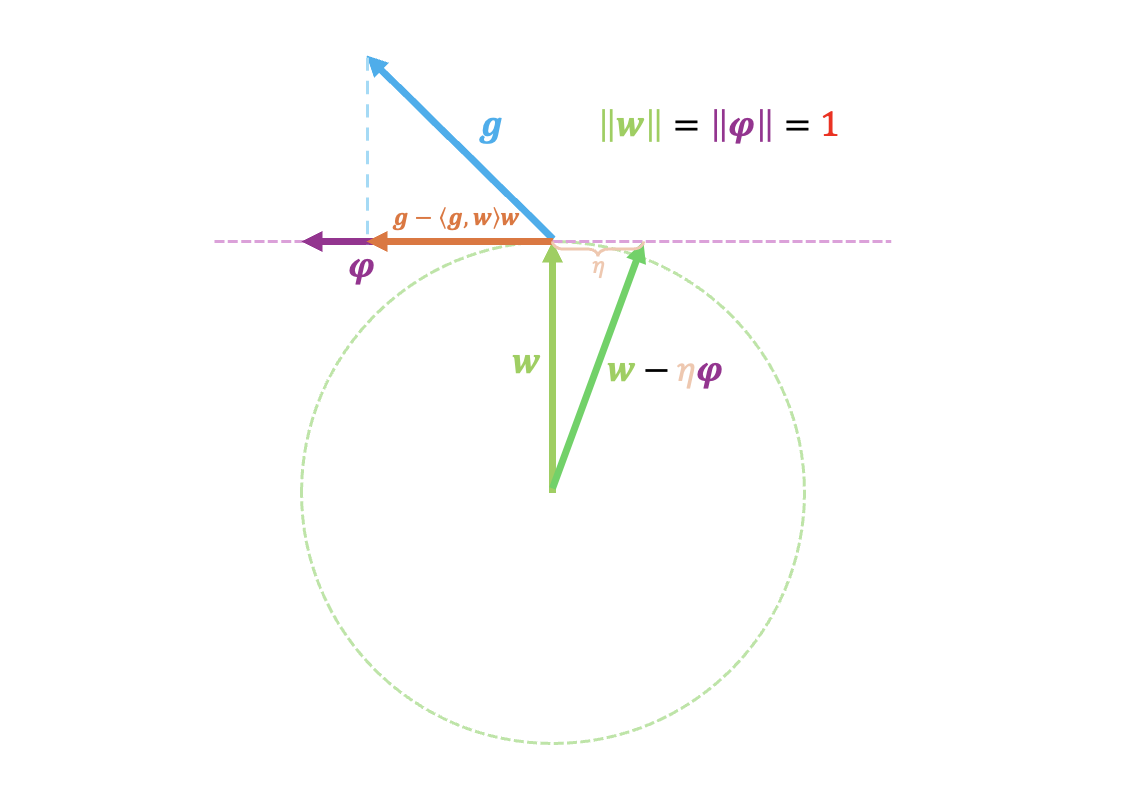
Many readers likely appreciate this geometric perspective; it is indeed aesthetically pleasing. However, I must remind you to prioritize understanding the algebraic solution process. Clear geometric meaning is often a luxury—it is something to be hoped for but not always found. In most cases, the complex algebraic process is the essence.
General Results
Some readers might want to generalize this to the general p-norm. Let’s try and see what difficulties arise. The problem becomes: \max_{\boldsymbol{\varphi}} \langle\boldsymbol{g},\boldsymbol{\varphi}\rangle \qquad \text{s.t.}\qquad \Vert\boldsymbol{\varphi}\Vert_p = 1,\,\,\Vert\boldsymbol{w}-\eta\boldsymbol{\varphi}\Vert_p = 1,\,\,\Vert\boldsymbol{w}\Vert_p=1 The first-order approximation converts \Vert\boldsymbol{w}-\eta\boldsymbol{\varphi}\Vert_p = 1 into \langle\boldsymbol{w}^{[p-1]},\boldsymbol{\varphi}\rangle = 0. Introducing the Lagrange multiplier \lambda: \langle\boldsymbol{g},\boldsymbol{\varphi}\rangle = \langle\boldsymbol{g},\boldsymbol{\varphi}\rangle + \lambda\langle\boldsymbol{w}^{[p-1]},\boldsymbol{\varphi}\rangle = \langle \boldsymbol{g} + \lambda\boldsymbol{w}^{[p-1]},\boldsymbol{\varphi}\rangle \leq \Vert\boldsymbol{g} + \lambda\boldsymbol{w}^{[p-1]}\Vert_q \Vert\boldsymbol{\varphi}\Vert_p = \Vert\boldsymbol{g} + \lambda\boldsymbol{w}^{[p-1]}\Vert_q The condition for equality is: \boldsymbol{\varphi} = \frac{(\boldsymbol{g} + \lambda\boldsymbol{w}^{[p-1]})^{[q/p]}}{\Vert(\boldsymbol{g} + \lambda\boldsymbol{w}^{[p-1]})^{[q/p]}\Vert_p} So far, there are no substantial difficulties. However, we then need to find \lambda such that \langle\boldsymbol{w}^{[p-1]},\boldsymbol{\varphi}\rangle = 0. When p \neq 2, this is a complex non-linear equation with no simple closed-form solution (though once solved, it guaranteed to be the optimal solution by Hölder’s inequality). Thus, for general p, we stop here and seek numerical methods when specific instances arise.
Besides p=2, we can consider p\to\infty. In this case, \boldsymbol{\varphi}=\mathop{\mathrm{sign}}(\boldsymbol{g} + \lambda\boldsymbol{w}^{[p-1]}). The condition \Vert\boldsymbol{w}\Vert_p=1 implies that the maximum of |w_1|, |w_2|, \dots, |w_n| is 1. If we further assume there is only one such maximum, then \boldsymbol{w}^{[p-1]} is a one-hot vector with \pm 1 at the position of the maximum absolute value and zero elsewhere. In this case, \lambda can be solved, and the result is to clip the gradient at the position of the maximum value to zero.
Summary
This article starts a new series focusing on "equality constraints" in optimization, attempting to find the "direction of steepest descent" for common constraints. As the first installment, we discussed the SGD variant under the "hypersphere" constraint.
Reprinting: Please include the original address of this article: https://kexue.fm/archives/11196
Further details on reprinting: Please refer to "Scientific Space FAQ".