Two weeks ago, I wrote “Aligning with Full Fine-Tuning! This is the Most Brilliant LoRA Improvement I’ve Seen (Part 1)” (it wasn’t numbered “Part 1” at the time). In that post, I introduced a LoRA variant called “LoRA-GA,” which improves the initialization of LoRA through gradient SVD to achieve alignment between LoRA and full fine-tuning. Of course, theoretically, this only aligns the weight W_1 after the first update step. At the time, some readers raised the question: “What about the subsequent W_2, W_3, \dots?” I hadn’t thought too deeply about it then, simply assuming that after aligning the first step, the subsequent optimization would follow a relatively optimal trajectory.
Interestingly, shortly after LoRA-GA was released, a new paper appeared on arXiv titled “LoRA-Pro: Are Low-Rank Adapters Properly Optimized?”. The proposed LoRA-Pro happens to answer this exact question! LoRA-Pro also aims to align with full fine-tuning, but it aligns the gradient at every step, thereby aligning the entire optimization trajectory. This serves as a perfectly complementary improvement to LoRA-GA.
Aligning with Full Fine-Tuning
This article continues using the notation and content from the previous post, so I will only provide a brief review here without detailed repetition. The parameterization of LoRA is: W = (W_0 - A_0 B_0) + AB where W_0 \in \mathbb{R}^{n\times m} is the pre-trained weight, A\in\mathbb{R}^{n\times r}, B\in\mathbb{R}^{r\times m} are the newly introduced trainable parameters, and A_0, B_0 are their initial values.
As mentioned in the previous post, full fine-tuning often outperforms LoRA, so full fine-tuning is the direction LoRA should most aim to align with. To describe this quantitatively, we write the optimization formulas for full fine-tuning and LoRA fine-tuning under SGD, respectively: W_{t+1} = W_t - \eta G_t and \begin{gathered} A_{t+1} = A_t - \eta G_{A,t} = A_t - \eta G_t B_t^{\top},\quad B_{t+1} = B_t - \eta G_{B,t} = B_t - \eta A_t^{\top}G_t \\[8pt] W_{t+1} = W_t - A_t B_t + A_{t+1} B_{t+1} \approx W_t - \eta(A_t A_t^{\top}G_t + G_tB_t^{\top} B_t) \end{gathered} where \mathcal{L} is the loss function, \eta is the learning rate, G_t=\frac{\partial \mathcal{L}}{\partial W_t}, G_{A,t}=\frac{\partial \mathcal{L}}{\partial A_t}=\frac{\partial \mathcal{L}}{\partial W_t} B_t^{\top}=G_t B_t^{\top}, and G_{B,t}=\frac{\partial \mathcal{L}}{\partial B_t}=A_t^{\top}\frac{\partial \mathcal{L}}{\partial W_t} =A_t^{\top}G_t.
The idea of LoRA-GA is that we should at least make W_1 of full fine-tuning and LoRA as similar as possible. Thus, it minimizes the objective: \mathop{\text{argmin}}_{A_0,B_0}\left\Vert A_0 A_0^{\top}G_0 + G_0 B_0^{\top} B_0 - G_0\right\Vert_F^2 The optimal solution can be obtained by performing SVD on G_0, allowing us to find the optimal A_0, B_0 as the initialization for A, B.
Step-by-Step Alignment
The idea of LoRA-Pro is more thorough: it hopes to align every W_t of full fine-tuning and LoRA. But how can this be achieved? Should we minimize \left\Vert A_t A_t^{\top}G_t + G_t B_t^{\top} B_t - G_t\right\Vert_F^2 at every step? This is clearly incorrect because A_t, B_t are determined by the optimizer based on A_{t-1}, B_{t-1} and their gradients; they are not freely adjustable parameters.
It seems there is nothing left to modify. However, LoRA-Pro cleverly realizes: since “A_t, B_t are determined by the optimizer based on A_{t-1}, B_{t-1} and their gradients,” and we cannot change the previous A_{t-1}, B_{t-1} or the gradients, we can still change the optimizer! Specifically, we change the update rules for A_t, B_t to: \begin{gathered} A_{t+1} = A_t - \eta H_{A,t} \\ B_{t+1} = B_t - \eta H_{B,t} \end{gathered} where H_{A,t}, H_{B,t} are to be determined, but their shapes match A and B. Now we can write: W_{t+1} = W_t - A_t B_t + A_{t+1} B_{t+1} \approx W_t - \eta(H_{A,t} B_t + A_t H_{B,t}) At this point, we can adjust H_{A,t}, H_{B,t} to make this W_{t+1} as close as possible to the W_{t+1} of SGD: \mathop{\text{argmin}}_{H_{A,t},H_{B,t}}\left\Vert H_{A,t} B_t + A_t H_{B,t} - G_t\right\Vert_F^2 Next, we solve this optimization problem. For simplicity, we omit the subscript t during the derivation, considering: \mathop{\text{argmin}}_{H_A,H_B}\left\Vert H_A B + A H_B - G\right\Vert_F^2\label{eq:loss}
Simplifying the Objective
Since there are no constraints between H_A and H_B, the optimization of H_A and H_B is independent. Therefore, we can adopt a strategy of optimizing H_A first and then H_B (or vice versa). When we optimize H_A, H_B is treated as a constant. To this end, we first consider the following simplified equivalent proposition: \mathop{\text{argmin}}_H\left\Vert H B - X\right\Vert_F^2\label{eq:h-xb-loss} where H\in\mathbb{R}^{n\times r}, B\in\mathbb{R}^{r\times m}, X\in\mathbb{R}^{n\times m}. If r=m and B is invertible, we can directly solve the equation HB=X, i.e., H=XB^{-1}. When r < m, we must resort to optimization. Noting that HB-X is linear with respect to H, this is essentially a least squares problem for linear regression, which has an analytical solution: H = XB^{\top}(B B^{\top})^{-1} \label{eq:h-xb} where B^{\top}(B B^{\top})^{-1} is the “pseudo-inverse” of matrix B. If you are unfamiliar with this answer, we can derive it on the spot. First, let l=\left\Vert H B - X\right\Vert_F^2. Taking the derivative with respect to H gives: \frac{\partial l}{\partial H} = 2(HB - X)B^{\top} = 2(HBB^{\top} - XB^{\top}) Setting it to zero yields equation [eq:h-xb]. Some readers might not be familiar with matrix calculus rules; however, according to the chain rule, it is easy to imagine that \frac{\partial l}{\partial H} is 2(HB - X) multiplied by B in some way. Since we require the shape of \frac{\partial l}{\partial H} to be the same as H (i.e., n\times r), the only way to construct an n\times r result from 2(HB - X) and B is 2(HB - X)B^{\top}.
Similarly, the derivative of \left\Vert AH - X\right\Vert_F^2 with respect to H is 2A^{\top}(AH - X), which leads to: \mathop{\text{argmin}}_H\left\Vert AH - X\right\Vert_F^2\quad\Rightarrow\quad H = (A^{\top} A)^{-1}A^{\top}X \label{eq:h-ax}
Complete Results
With the conclusions from [eq:h-xb] and [eq:h-ax], we can proceed to solve [eq:loss]. First, we fix H_B. According to equation [eq:h-xb], we get: H_A = (G - A H_B) B^{\top}(B B^{\top})^{-1}\label{eq:h-a-1} Note that the objective function in [eq:loss] possesses an invariance: \left\Vert H_A B + A H_B - G\right\Vert_F^2 = \left\Vert (H_A + AC) B + A (H_B - CB) - G\right\Vert_F^2 where C is any r\times r matrix. In other words, the solution for H_A can be added/subtracted by any matrix of the form AC, as long as H_B is subtracted/added by the corresponding CB. Using this property, we can simplify H_A in equation [eq:h-a-1] to: H_A = G B^{\top}(B B^{\top})^{-1} Substituting this back into the objective function gives: \mathop{\text{argmin}}_{H_B}\left\Vert A H_B - G(I - B^{\top}(B B^{\top})^{-1}B)\right\Vert_F^2 According to equation [eq:h-ax], we get: H_B = (A^{\top} A)^{-1}A^{\top}G(I - B^{\top}(B B^{\top})^{-1}B) Noticing that G B^{\top} and A^{\top}G are exactly the gradients G_A and G_B of A and B, and again utilizing the aforementioned invariance, we can write the complete solution: \left\{\begin{aligned} H_A =&\, G_A (B B^{\top})^{-1} + AC \\ H_B =&\, (A^{\top} A)^{-1}G_B(I - B^{\top}(B B^{\top})^{-1}B) - CB \end{aligned}\right.
Optimal Parameters
So far, we have derived the forms of H_A and H_B, but the solution is not unique due to the freely selectable parameter matrix C. We can choose an appropriate C to make the final H_A, H_B possess certain desired characteristics.
For example, currently H_A and H_B are somewhat asymmetric, with H_B having the extra term -(A^{\top} A)^{-1}G_B B^{\top}(B B^{\top})^{-1}B. We can distribute this term equally between H_A and H_B to make them more symmetric, which is equivalent to choosing C = -\frac{1}{2}(A^{\top} A)^{-1}G_B B^{\top}(B B^{\top})^{-1}: \left\{\begin{aligned} H_A =&\, \left[I - \frac{1}{2}A(A^{\top}A)^{-1}A^{\top}\right]G_A (B B^{\top})^{-1} \\ H_B =&\, (A^{\top} A)^{-1}G_B\left[I - \frac{1}{2}B^{\top}(B B^{\top})^{-1}B\right] \end{aligned}\right. This C is also the solution to the following two optimization problems: \begin{aligned} &\,\mathop{\text{argmin}}_C \Vert H_A B - A H_B\Vert_F^2 \\ &\,\mathop{\text{argmin}}_C \Vert H_A B - G\Vert_F^2 + \Vert A H_B - G\Vert_F^2 \\ \end{aligned} The first objective can be understood as making the contributions of A and B to the final effect as equal as possible, which shares some similarities with the hypothesis in “Can LoRA Gain a Bit More by Configuring Different Learning Rates?”. The second objective is to make both H_A B and A H_B as close to the full gradient G as possible. Taking l=\Vert H_A B - A H_B\Vert_F^2 as an example, the derivative is: \frac{\partial l}{\partial C} = 4A^{\top}(H_A B - A H_B)B^{\top}=4A^{\top}\left[G_A (BB^{\top})^{-1}B + 2ACB\right]B^{\top} Setting it to zero allows us to solve for the same C. The two key steps in the simplification are [I - B^{\top}(B B^{\top})^{-1}B]B^{\top} = 0 and A^{\top}G_A = G_B B^{\top}.
LoRA-Pro chooses a slightly different C, which is the optimal solution to the following objective function: \mathop{\text{argmin}}_C \Vert H_A - G_A\Vert_F^2 + \Vert H_B - G_B\Vert_F^2 The intention here is also clear: H_A, H_B are used to replace G_A, G_B. If the same effect can be achieved, it is a reasonable choice to keep the changes relative to G_A, G_B as small as possible. Similarly, taking the derivative with respect to C and setting it to zero, we get: A^{\top}A C + C B B^{\top} = -A^{\top} G_A (BB^{\top})^{-1} Now we have an equation for C. This type of equation is called a “Sylvester equation.” While an analytical solution for C can be written using Kronecker products, it is unnecessary because the complexity of numerical solvers is lower than that of the analytical solution. Overall, these selection schemes for C are all aimed at making H_A, H_B more symmetric from some perspective. Although I haven’t personally conducted comparative experiments, I believe there won’t be significant differences between these choices.
General Discussion
Let’s summarize the results obtained so far. Our model is still a standard LoRA, but the goal is to make every update step approximate the result of full fine-tuning. To this end, we assumed the optimizer is SGD and compared the W_{t+1} obtained by full fine-tuning and LoRA given the same W_t. We found that to achieve this goal, the gradients G_A, G_B of A, B in the update process need to be replaced by the H_A, H_B derived above.
Next, we return to a common issue in optimization analysis: the previous analysis was based on the SGD optimizer, but in practice, we more commonly use Adam. How should we modify it? If we repeat the derivation for the Adam optimizer, the result is that the gradient G in H_A, H_B should be replaced by the update direction U of Adam under full fine-tuning. However, U needs to be calculated from the full fine-tuning gradient G according to Adam’s update rules. In our LoRA scenario, we cannot obtain the full fine-tuning gradient; we only have the gradients G_A, G_B of A, B.
However, we can consider an approximate scheme. Since the optimization objective of H_A B + A H_B is to approximate G, we can use it as an approximation of G to execute Adam. This makes the entire process feasible. Thus, we can write the following update rules: \begin{array}{l} \begin{array}{l}G_A = \frac{\partial\mathcal{L}}{\partial A_{t-1}},\,\,G_B = \frac{\partial\mathcal{L}}{\partial B_{t-1}}\end{array} \\ \color{green}{\left.\begin{array}{l}H_A = G_A (B B^{\top})^{-1} \\ H_B = (A^{\top} A)^{-1}G_B(I - B^{\top}(B B^{\top})^{-1}B) \\ \tilde{G} = H_A B + A H_B \end{array}\quad\right\} \text{Estimate Gradient}} \\ \color{red}{\left.\begin{array}{l}M_t = \beta_1 M_{t-1} + (1 - \beta_1) \tilde{G} \\ V_t = \beta_2 V_{t-1} + (1 - \beta_2) \tilde{G}^2 \\ \hat{M}_t = \frac{M_t}{1-\beta_1^t},\,\,\hat{V}_t = \frac{V_t}{1-\beta_2^t},\,\,U = \frac{\hat{M}_t}{\sqrt{\hat{V}_t + \epsilon}}\end{array}\quad\right\} \text{Adam Update}} \\ \color{purple}{\left.\begin{array}{l}U_A = UB^{\top},\,\, U_B = A^{\top} U \\ \tilde{H}_A = U_A (B B^{\top})^{-1} + AC \\ \tilde{H}_B = (A^{\top} A)^{-1}U_B(I - B^{\top}(B B^{\top})^{-1}B) - CB \end{array}\quad\right\} \text{Project to } A, B} \\ \begin{array}{l}A_t = A_{t-1} - \eta \tilde{H}_A \\ B_t = B_{t-1} - \eta \tilde{H}_B \\ \end{array} \\ \end{array} This is the final update algorithm used by LoRA-Pro (more accurately, LoRA-Pro uses AdamW, which is slightly more complex but not substantially different). However, setting aside the extra complexity introduced by these changes, the biggest problem with this algorithm is that the moving average variables M, V are full-rank, just like in full fine-tuning. This means the optimizer does not save memory compared to full fine-tuning; it only saves some memory for parameters and gradients through low-rank decomposition. This is a significant increase in memory consumption compared to conventional LoRA.
A simpler scheme (which I haven’t tested) would be to directly replace G_A, G_B with H_A, H_B and then calculate according to the standard LoRA Adam update rules. This way, the shapes of M, V would match A, B, maximizing memory savings. However, the theoretical foundation for Adam in this case would not be as strong as LoRA-Pro’s Adam, relying more on the “faith” that conclusions from SGD can be applied in parallel to Adam, similar to LoRA-GA.
Experimental Results
The experimental results of LoRA-Pro on GLUE are even more impressive, surpassing the results of full fine-tuning:
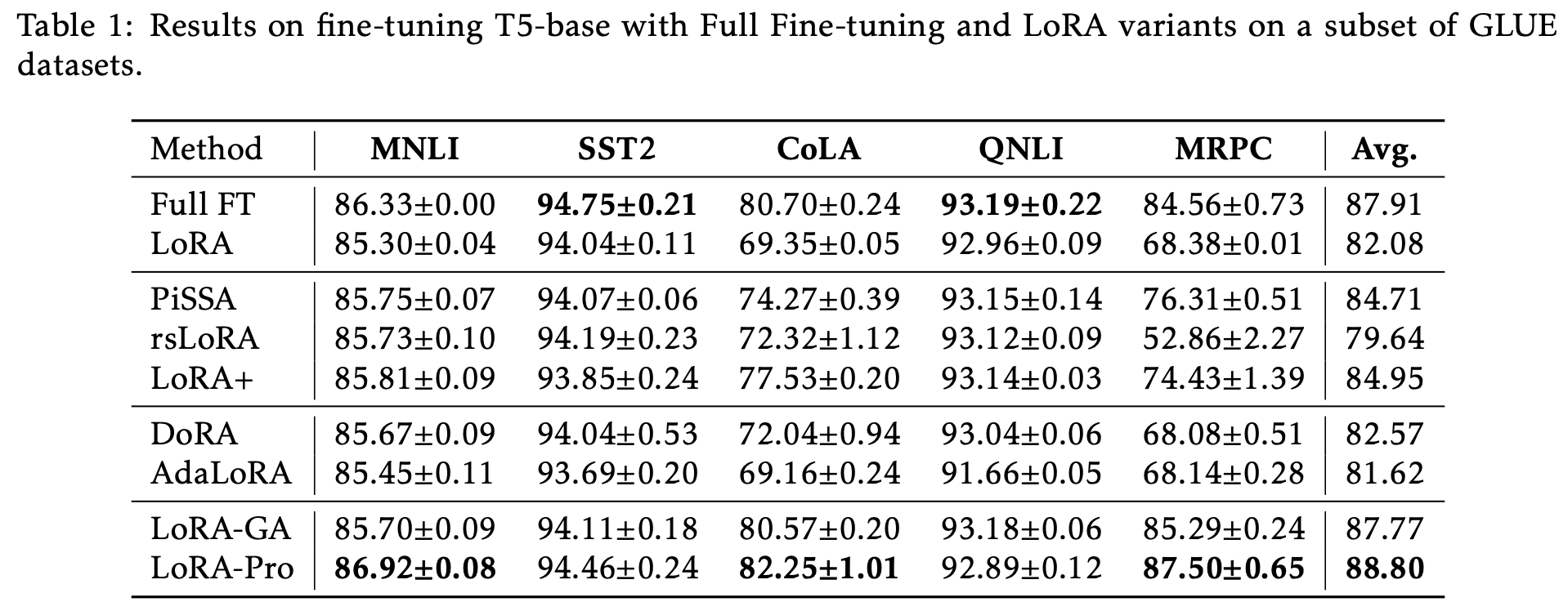
However, the paper only includes this experiment. It seems LoRA-Pro was written in a bit of a hurry, perhaps because the authors felt a strong sense of “collision” after seeing LoRA-GA and wanted to stake their claim first. When I first saw LoRA-Pro, my first reaction was also that it collided with LoRA-GA, but upon careful reading, I found that they are actually complementary results under the same core idea.
From the results of LoRA-Pro, it involves the inversion of A^{\top} A and B B^{\top}, so it is clear that at least one of A or B cannot be initialized to zero. A more intuitive choice is orthogonal initialization, making the initial A^{\top} A and B B^{\top} (multiples of) the identity matrix. As we saw in Part 1, the initialization provided by LoRA-GA is exactly an orthogonal initialization. Thus, LoRA-Pro and LoRA-GA can be considered a “perfect pair.”
Summary
This article introduced another work on aligning with full fine-tuning, LoRA-Pro. It and the previously discussed LoRA-GA are complementary results. LoRA-GA attempts to align LoRA with full fine-tuning by improving initialization, while LoRA-Pro is more thorough, modifying the optimizer’s update rules to ensure every step of LoRA’s update aligns as closely as possible with full fine-tuning. Both are brilliant improvements to LoRA and are truly a pleasure to study.
Reprinting: Please include the original address of this article: https://kexue.fm/archives/10266
Further details on reprinting: Please refer to: Scientific Space FAQ