Monarch Matrices: Computationally Efficient Sparse Matrix Decomposition

Permutation Matrix

The permutation matrix P achieves the effect of permuting the vector [x_1, x_2, \cdots, x_n] into a new vector: \begin{equation} [x_1, x_{1+m}, \cdots , x_{1+(m-1)m}, x_2, x_{2+m}, \cdots , x_{2+(m-1)m}, \cdots , x_m, x_{2m}, \cdots , x_n] \end{equation} While this notation might seem confusing, the implementation in code is actually very simple:

Px = x.reshape(m, m).transpose().reshape(n)

As shown in the figure below:

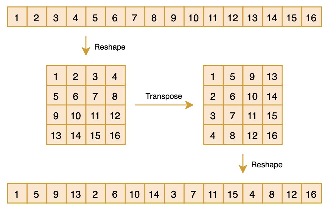
Readers with a background in Computer Vision (CV) might find this operation familiar; it is essentially the "Shuffle" operation in ShuffleNet. This combination of reshaping, transposing, and reshaping back to the original size creates a "pseudo-shuffle" effect. It can also be viewed as an m-ary "bit-reversal permutation." Obviously, performing this operation twice restores the vector to its original state, so we have P^2 = I, which implies P^{-1} = P^{\top} = P.

Block Diagonal

After discussing P, let’s look at L and R. They are also n \times n matrices, but they are block-diagonal matrices with m \times m blocks. Each block is of size m \times m, as shown below:

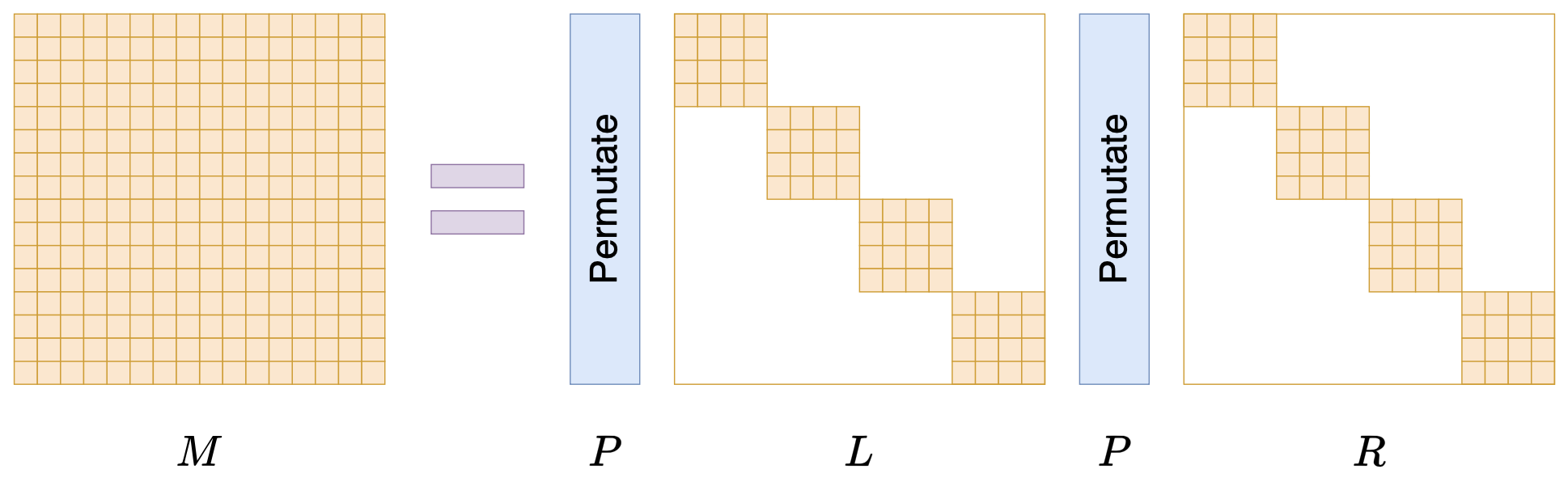
When n is sufficiently large, the number of zeros in L and R dominates, so both L and R are sparse matrices. Thus, the Monarch matrix is a matrix decomposition form with sparse characteristics. Since P is fixed, the variable elements in PLPR come from the non-zero elements of L and R. Therefore, although M is an n \times n matrix, it actually has no more than 2m^3 = 2n^{1.5} free parameters. From the exponent 1.5, we can see the intent of Monarch matrices: they aim to reduce operations that originally required quadratic complexity to 1.5-power complexity through Monarch matrix approximation.

Efficiency Analysis

Can Monarch matrices achieve this goal? In other words, do they meet the "practical" standard mentioned earlier? We will discuss expressiveness later; let’s first look at computational efficiency.

For example, in "matrix-vector" multiplication, the standard complexity is \mathcal{O}(n^2). However, for a Monarch matrix, we have Mx = P(L(P(Rx))). Since multiplying by P involves only simple reshaping and transposing, it consumes almost no computation. The main computational load comes from multiplying L or R with a vector. Due to the block-diagonal nature of L and R, we can divide the vector into m groups, transforming the operation into m multiplications of m \times m matrices with m-dimensional vectors. The total complexity is 2m \times \mathcal{O}(m^2) = \mathcal{O}(2n^{1.5}), which is lower than \mathcal{O}(n^2).

Consider matrix inversion M^{-1}x. The standard complexity for inverting an n-th order matrix is \mathcal{O}(n^3). For a Monarch matrix, we have M^{-1}x = R^{-1}PL^{-1}Px. The main computational load comes from L^{-1}, R^{-1}, and the corresponding matrix-vector multiplications. Since L and R are block-diagonal, we only need to invert each block matrix on the diagonal. This involves inverting 2m matrices of size m \times m, with a complexity of 2m \times \mathcal{O}(m^3) = \mathcal{O}(2n^2), which is also lower than the standard \mathcal{O}(n^3). It is also possible to write out M^{-1} explicitly, but this requires using the identity in equation [eq:high-m-lr].

In conclusion, because multiplication by P is computationally negligible and L, R are block-diagonal, operations involving n-th order Monarch matrices can basically be transformed into 2m independent operations on m \times m matrices, thereby reducing the total computational complexity. Thus, Monarch matrices are certainly efficient, and since the non-zero elements of L and R already have a square structure, they are easy to implement and can fully utilize GPUs without unnecessary waste.

High-Dimensional Arrays

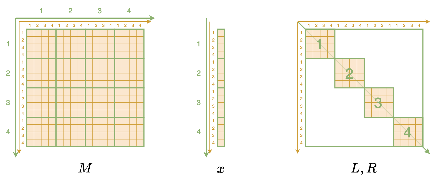
The key to understanding this algorithm is to transform Monarch-related matrices and vectors into higher-dimensional array forms. Specifically, the Monarch matrix M is originally a 2D array where each element M_{i,j} represents the element at the i-th row and j-th column. Now, based on the characteristics of block matrices, we represent it equivalently as a 4D array. Each element M_{i,j,k,l} represents the element in the i-th large row, j-th small row, k-th large column, and l-th small column, as shown below:

While it sounds complicated, the code is just one line:

M.reshape(m, m, m, m)

Similarly, an n-dimensional (column) vector x is converted into m \times m 2D data with x.reshape(m, m). Naturally, L and R are represented as m \times m \times m 3D arrays, where L_{i,j,k} represents the element in the i-th block, j-th small row, and k-th small column. This is already the most efficient way to store L and R, but for unified processing, we can also use the Kronecker delta symbol to lift them to 4D, e.g., L_{i,j,k,l} = \delta_{i,k}L_{i,j,l} and R_{i,j,k,l} = \delta_{i,k}R_{i,j,l}.

A New Identity

Next, we will derive a new relationship between M and L, R. First, it can be proven that in the 2D representation, the multiplication of matrix P and vector x becomes simpler: the result is the transpose of x, i.e., (Px)_{i,j} = x_{j,i}. Therefore, we have (PR)_{i,j,k,l} = R_{j,i,k,l} = \delta_{j,k}R_{j,i,l}. Then, for the multiplication of two matrices in 4D representation, there are two summation indices: \begin{equation} (L P R)_{\alpha,\beta,k,l} = \sum_{i,j} L_{\alpha,\beta,i,j}(PR)_{i,j,k,l} = \sum_{i,j} \delta_{\alpha, i} L_{\alpha,\beta,j}\delta_{j,k}R_{j,i,l} = L_{\alpha,\beta,k}R_{k,\alpha,l} \end{equation} Finally, (P L P R)_{\alpha,\beta,k,l} = L_{\beta,\alpha,k}R_{k,\beta,l}. Replacing \alpha, \beta back with i, j, we get (P L P R)_{i,j,k,l} = L_{j,i,k}R_{k,j,l}. Since M = PLPR, we have: \begin{equation} M_{i,j,k,l} = L_{j,i,k}R_{k,j,l} \label{eq:high-m-lr} \end{equation} From this equation, we can see that when we fix a pair (j,k), the left side is a submatrix and the right side is the outer product of two vectors. This means that if we want to find the Monarch approximation for matrix A, we only need to convert A into a 4D array in the same way and fix a pair (j,k). The problem then becomes finding the "rank-1 approximation" of the corresponding submatrix! In other words, with this identity, finding the Monarch approximation of matrix A can be transformed into finding the "rank-1 approximation" of m^2 submatrices. This can be done using SVD, with each sub-problem having a complexity not exceeding \mathcal{O}(m^3), resulting in a total complexity not exceeding m^2 \times \mathcal{O}(m^3) = \mathcal{O}(n^{2.5}).

Reference Implementation

A simple reference implementation using Numpy is as follows:

import numpy as np

def monarch_factorize(A):
    m = int(np.sqrt(A.shape[0]))
    M = A.reshape(m, m, m, m).transpose(1, 2, 0, 3)
    U, S, V = np.linalg.svd(M)
    L = (U[:, :, :, 0] * S[:, :, :1]**0.5).transpose(0, 2, 1)
    R = (V[:, :, 0] * S[..., :1]**0.5).transpose(1, 0, 2)
    return L, R

def convert_3D_to_2D(LR, m, n):
    X = np.zeros((m, m, m, m))
    for i in range(m):
        X[i, i] += LR[i]
    return X.transpose(0, 2, 1, 3).reshape(n, n)

m = 8
n = m**2
A = np.where(np.random.rand(n, n) > 0.8, np.random.randn(n, n), 0)

L, R = monarch_factorize(A)
L_2d = convert_3D_to_2D(L, m, n)
R_2d = convert_3D_to_2D(R, m, n)

# P matrix implementation via reshape/transpose
def apply_P(X, m):
    n = m*m
    return X.reshape(m, m, n).transpose(1, 0, 2).reshape(n, n)

PL = apply_P(L_2d, m)
PR = apply_P(R_2d, m)

U, S, V = np.linalg.svd(A)

print('Monarch error:', np.square(A - PL.dot(PR)).mean())
print('Low-Rank error:', np.square(A - (U[:, :m] * S[:m]).dot(V[:m])).mean())

I briefly compared the rank-m approximation obtained by SVD (where the parameter count is comparable to the Monarch approximation). I found that for completely dense matrices, the mean squared error of the rank-m approximation is often better than the Monarch approximation (though not by much). This is expected, as the Monarch approximation algorithm is essentially a customized version of SVD. However, if the matrix to be approximated is sparse, the Monarch approximation error is often better, and the sparser the matrix, the better the performance.

Non-Square Orders

To this end, we first introduce some notation. Let b be a factor of n. \mathcal{BD}^{(b,n)} denotes the set of all \frac{n}{b} \times \frac{n}{b} block-diagonal matrices where each block is a b \times b submatrix. This is clearly a generalization of the previous L and R; using this notation, we can write L, R \in \mathcal{BD}^{(\sqrt{n},n)}. Furthermore, we need to generalize the permutation matrix P. Previously, we said P is implemented as Px = x.reshape(m, m).transpose().reshape(n). Now we generalize this to Px = x.reshape(n // b, b).transpose().reshape(n), denoted as P_{(\frac{n}{b},b)}.

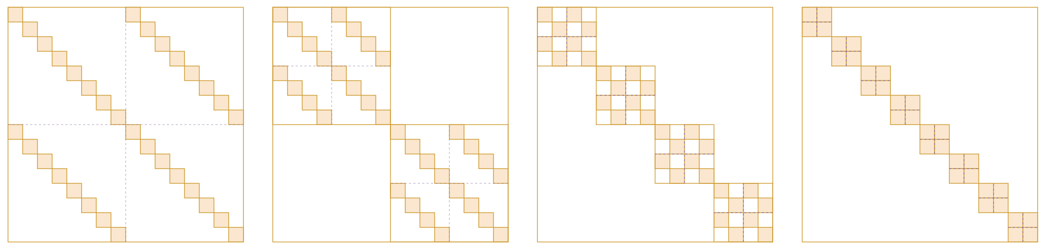
With these notations, we can define general Monarch matrices (from the original paper’s appendix): \begin{equation} \mathcal{M}^{(b,n)} = \Bigg\{M = P_{(b,\frac{n}{b})} L P_{(\frac{n}{b},b)} R\,\Bigg|\, L\in\mathcal{BD}^{(\frac{n}{b},n)}, R\in\mathcal{BD}^{(b,n)} \Bigg\} \end{equation} The schematic is as follows:

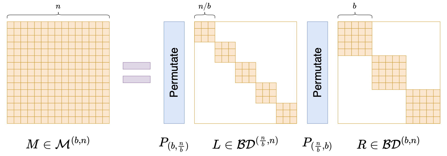
The Monarch matrix defined earlier can be simply denoted here as \mathcal{M}^{(n)} = \mathcal{M}^{(\sqrt{n},n)}. It is not difficult to calculate that L has at most \frac{n^2}{b} non-zero elements, and R has at most nb non-zero elements. The total is \frac{n^2}{b} + nb, which reaches its minimum at b = \sqrt{n}. Thus, b = \sqrt{n} is one of the sparsest examples.

Focusing on Form

Readers might wonder why we distinguish between L \in \mathcal{BD}^{(\frac{n}{b},n)} and R \in \mathcal{BD}^{(b,n)}. Why not use the same for both? In fact, this design is intended to keep the identity in equation [eq:high-m-lr] valid in high-dimensional representation, allowing for a similar decomposition algorithm and theoretically guaranteeing its expressiveness.

If we do not care about these theoretical details and only wish to construct a matrix parameterization with sparse characteristics, we can generalize Monarch matrices more flexibly, for example: \begin{equation} M = \left(\prod_{i=1}^k P_i B_i\right)P_0 \end{equation} where B_1, B_2, \cdots, B_k \in \mathcal{BD}^{(b,n)}, and P_0, P_1, \cdots, P_k are all permutation matrices. Multiplying by P_0 at the end is for symmetry and is not strictly necessary. If you find it necessary, you can even choose different b for each B_i, i.e., B_i \in \mathcal{BD}^{(b_i,n)}.

Furthermore, you can combine the form of low-rank decomposition to generalize to non-square block matrices, as shown below:

Based on this analogy, we can further extend the concept of Monarch matrices to non-square matrices. In short, if one only needs a sparse structured matrix similar to a Monarch matrix and does not care about theoretical details, the possibilities are limited only by our imagination.