Revisiting SSM (IV): A New Perspective from Rational Generating Functions

Background Review

First, let’s briefly review the results of our discussion on S4 from the previous article. S4 is based on the following linear RNN: \begin{equation} \begin{aligned} x_{k+1} =&\, \bar{A} x_k + \bar{B} u_k \\ y_{k+1} =&\, \bar{C}^* x_{k+1} \\ \end{aligned} \label{eq:linear} \end{equation} where u, y \in \mathbb{R}, x \in \mathbb{R}^d, \bar{A} \in \mathbb{R}^{d \times d}, and \bar{B}, \bar{C} \in \mathbb{R}^{d \times 1}. Here, we aim for a general discussion, so we bypass the connection between \bar{A} and A and assume \bar{A} is a general matrix. Assuming the initial state is zero, direct iteration yields: \begin{equation} y_L = \sum_{k=0}^L \bar{C}^*\bar{A}^k \bar{B}u_{L-k} = \bar{K}_{< L} * u_{< L} \end{equation} where * denotes the convolution operation, and \begin{equation} \bar{K}_k = \bar{C}^*\bar{A}^k\bar{B},\quad \bar{K}_{< L} = \big(\bar{K}_0, \bar{K}_1, \cdots, \bar{K}_{L-1}\big),\quad u_{< L} = (u_0, u_1, \cdots, u_{L-1}) \end{equation} Since convolution can be computed efficiently via the Discrete Fourier Transform (DFT), the remaining problem is how to compute \bar{K} efficiently. This is the core contribution of S4. To this end, S4 introduces the generating function: \begin{align} \mathcal{G}(z|\bar{K}) =&\, \sum_{k=0}^{\infty} \bar{C}^*\bar{A}^k \bar{B}z^k = \bar{C}^*\left(I - z\bar{A}\right)^{-1}\bar{B} \\ \mathcal{G}_L(z|\bar{K}) =&\, \sum_{k=0}^{L-1} \bar{C}^*\bar{A}^k \bar{B}z^k = \bar{C}^*(I - z^L\bar{A}^L)\left(I - z\bar{A}\right)^{-1}\bar{B} \end{align} If \mathcal{G}_L(z|\bar{K}) can be computed efficiently, we can substitute z=e^{-2i\pi l/L}, l=0,1,2,\dots,L-1, and the results will be the DFT of \bar{K}. Further Inverse DFT (IDFT) then yields \bar{K}. Since z at these points always satisfies z^L=1, we can also set \tilde{C}^* = \bar{C}^*(I - \bar{A}^L), making the form of \mathcal{G}_L(z|\bar{K}) identical to \mathcal{G}(z|\bar{K}): \begin{equation} \mathcal{G}_L(z|\bar{K}) = \tilde{C}^*\left(I - z\bar{A}\right)^{-1}\bar{B} \end{equation}

How can \mathcal{G}(z|\bar{K}) or \mathcal{G}_L(z|\bar{K}) be computed efficiently? S4 decomposes \bar{A} into a "diagonal + low-rank" form and then uses the Woodbury identity for calculation. The final result is: \begin{equation} \mathcal{G}(z|\bar{K}) = \frac{2}{1+z}\bar{C}^* \left[R_z^{-1} - R_z^{-1}u(I + v^*R_z^{-1}u)^{-1} v^*R_z^{-1}\right]B \end{equation} where R_z is a d \times d diagonal matrix, and u, v, B, \bar{C} are all d \times 1 column vectors. This means that for a given z, the complexity of computing \mathcal{G}(z|\bar{K}) is \mathcal{O}(d). If we need to compute this for z=e^{-2i\pi l/L}, l=0,1,2,\dots,L-1, a naive implementation would require \mathcal{O}(Ld) computation. S4 proposes transforming this into a Cauchy kernel problem, further reducing the complexity to \mathcal{O}((L+d)\log^2(L+d)).

Regardless of the method, we find that the complexity depends not only on L but also on d (the state size). RFT, however, proposes a new method that reduces the complexity directly to the ideal \mathcal{O}(L\log L), independent of the state size. Moreover, the derivation process is significantly simpler than S4 and does not rely on the assumption that \bar{A} is diagonal or "diagonal + low-rank."

Rational Functions

RFT stands for Rational Transfer Function, and its focus is on the Rational Function (the quotient of two polynomials). What is its relationship with generating functions? The authors of RFT brilliantly observed that \mathcal{G}_L(z|\bar{K}) is actually a rational function! Specifically, we have: \begin{equation} \mathcal{G}_L(z|\bar{K}) = \tilde{C}^*\left(I - z\bar{A}\right)^{-1}\bar{B} = \frac{b_1 + b_2 z + b_3 z^2 + \cdots + b_dz^{d-1}}{1 + a_1 z + a_2 z^2 + \cdots + a_d z^d} \label{eq:gz-rf} \end{equation} where a_1, a_2, \cdots, a_d, b_1, b_2, \cdots, b_d are scalars. If \bar{A}, \bar{B}, \tilde{C} are all real matrices, then these are real numbers. To realize that such an equivalent form exists, we only need to use a classic formula for matrix inversion: \begin{equation} M^{-1} = \frac{\text{adj}(M)}{\det(M)} \end{equation} where \det(M) is the determinant of M, and \text{adj}(M) is the adjugate matrix of M. Since the adjugate matrix involves a large number of determinant calculations, this inversion formula is usually of little value in practical computation, but it often works wonders in theoretical analysis. For example, substituting it into \mathcal{G}_L(z|\bar{K}), we get: \begin{equation} \mathcal{G}_L(z|\bar{K}) = \tilde{C}^*\left(I - z\bar{A}\right)^{-1}\bar{B} = \frac{\tilde{C}^*\text{adj}(I - z\bar{A})\bar{B}}{\det(I - z\bar{A})} \end{equation} We know that a d-th order determinant is a sum of products of d elements, so \det(I - z\bar{A}) is a polynomial of degree d in z. Next, according to the definition of the adjugate matrix, each of its elements is a (d-1)-th order determinant, which is a polynomial of degree d-1. Multiplying by \tilde{C}^* on the left and \bar{B} on the right is merely a weighted sum of these elements, so the result is still a polynomial of degree d-1. Therefore, \mathcal{G}_L(z|\bar{K}) is a (d-1)-degree polynomial in z divided by a d-degree polynomial in z. By normalizing the constant term of the denominator to 1, we obtain Equation [eq:gz-rf].

Correspondence

Furthermore, we can use a determinant identity to determine the relationship between the coefficients a=(a_1, a_2, \cdots, a_d), b=(b_1, b_2, \cdots, b_d) and \bar{A}, \bar{B}, \tilde{C}. This identity is: \begin{equation} \det(I + UV) = \det(I + VU) \label{eq:det-iuv} \end{equation} Proving this determinant identity is not difficult; it is a common problem in graduate entrance exams. One only needs to notice that: \begin{equation} \begin{pmatrix}I & U \\ -V & I\end{pmatrix} = \begin{pmatrix}I + UV & U \\ 0 & I\end{pmatrix}\begin{pmatrix}I & 0 \\ -V & I\end{pmatrix} = \begin{pmatrix}I & 0 \\ -V & I + VU\end{pmatrix}\begin{pmatrix}I & U \\ 0 & I\end{pmatrix} \end{equation} According to the definition and form of the determinant, the determinant of the middle part is \det(I + UV), and the determinant of the rightmost part is \det(I + VU). They are determinants of the same matrix, so the results are equal. This result can be further generalized to (when A and D are invertible): \begin{equation} \det\begin{pmatrix}A & B \\ C & D\end{pmatrix} = \det(A)\det(D-CA^{-1}B) = \det(D)\det(A-BD^{-1}C) \end{equation} Going a bit further, it can also be generalized to the "Schur complement" theory, which we mentioned in "KL Divergence, Bhattacharyya Distance, and W-Distance of Two Multivariate Normal Distributions".

Returning to the main topic, note that in Equation [eq:det-iuv] and its derivation, we do not need to assume that U and V are square matrices. Thus, Equation [eq:det-iuv] actually holds for non-square matrices, as long as the identity matrix I automatically matches the size of UV and VU. Specifically, if U and V are column and row vectors respectively, then VU is a scalar, the corresponding I is 1, and its determinant is itself, i.e., \det(I + UV) = 1 + VU. Using this special case, we have: \begin{equation} \begin{aligned} \mathcal{G}_L(z|\bar{K}) =&\, z^{-1}\left[1+\tilde{C}^*\left(z^{-1}I - \bar{A}\right)^{-1}\bar{B} - 1 \right]\\ =&\, z^{-1}\left[\det\left(I + \left(z^{-1} I - \bar{A}\right)^{-1}\bar{B}\tilde{C}^*\right) - 1\right]\\ =&\, z^{-1}\left\{\det\left[\left(z^{-1} I - \bar{A}\right)^{-1}\left(z^{-1} I - \bar{A} + \bar{B}\tilde{C}^*\right)\right] - 1\right\} \\ =&\, z^{-1}\left[\frac{\det(z^{-1} I - \bar{A} + \bar{B}\tilde{C}^*)}{\det(z^{-1} I - \bar{A})} - 1\right] \\ =&\, \frac{z^{d-1}\left[\det(z^{-1} I - \bar{A} + \bar{B}\tilde{C}^*)-\det(z^{-1} I - \bar{A})\right]}{z^d\det(z^{-1} I - \bar{A})} \\ \end{aligned} \end{equation} The term \det(z^{-1} I - \bar{A}) in the denominator is the characteristic polynomial of the matrix \bar{A} with \lambda=z^{-1} as the variable. It is a monic polynomial of degree d in z^{-1}. After multiplying by z^d, it becomes a polynomial of degree d in z with a constant term of 1. Similarly, \det(z^{-1} I - \bar{A} + \bar{B}\tilde{C}^*) in the numerator is the characteristic polynomial of \bar{A} - \bar{B}\tilde{C}^* (a monic polynomial of degree d in z^{-1}). Subtracting \det(z^{-1} I - \bar{A}) yields a polynomial of degree d-1 in z^{-1}, which becomes a polynomial of degree d-1 in z after multiplying by z^{d-1}. Therefore, the vector a consists of the coefficients of the polynomial \det(\lambda I - \bar{A}) excluding the highest-degree term, while the vector b consists of the coefficients of the polynomial \det(\lambda I - \bar{A} + \bar{B}\tilde{C}^*) - \det(\lambda I - \bar{A}) (sorted from highest to lowest degree).

A Sudden Surprise

Now let’s pause and think about what we have done and where we are going.

Our starting point was the linear system [eq:linear]. To make it parallelizable for training, we transformed it into a convolution of \bar{K}_{< L} and u_{< L}, which can be computed efficiently by performing DFT, multiplying, and then performing IDFT. Thus, the efficiency of this step is not an issue. Now u_{< L} is available, but \bar{K}_{< L} is unknown. The problem becomes how to efficiently compute the convolution kernel \bar{K}_{< L} = \{\tilde{C}^*\bar{A}^k\bar{B}\}_{k=0}^{L-1}. To this end, we introduced the generating function \mathcal{G}_L(z|\bar{K}). As long as we can compute \mathcal{G}_L(z|\bar{K}) efficiently, we have: \begin{equation} DFT(\bar{K}_{< L}) = \Big\{\mathcal{G}_L(z|\bar{K})\Big\}_{z=e^{-2i\pi l/L}, l=0,1,2,\dots,L-1} \end{equation} Then IDFT can recover the original \bar{K}_{< L}. For z=e^{-2i\pi l/L}, we have z^L=1, so: \begin{equation} \mathcal{G}_L(z|\bar{K}) = \tilde{C}^*(I - z^L\bar{A}^L)\left(I - z\bar{A}\right)^{-1}\bar{B} = \underbrace{\bar{C}^*(I - \bar{A}^L)}_{\tilde{C}^*}\left(I - z\bar{A}\right)^{-1}\bar{B} \end{equation} That is, we can treat the entire \bar{C}^*(I - \bar{A}^L) as a trainable parameter \tilde{C}^* and solve for the corresponding \bar{C} for inference later.

S4 computes \mathcal{G}_L(z|\bar{K}) through "diagonal + low-rank" decomposition, while this paper points out that \mathcal{G}_L(z|\bar{K}) is actually a rational function, as in Equation [eq:gz-rf]. If we substitute z=e^{-2i\pi l/L} at this point, we find some surprising results. For example, the denominator: \begin{equation} 1 + a_1 z + a_2 z^2 + \cdots + a_d z^d = \sum_{k=0}^L a_k z^k = \sum_{k=0}^L a_k e^{-2i\pi kl/L} = DFT(\bar{a}_{< L}) \end{equation} where \bar{a}_{< L} = (a_0, a_1, a_2, \cdots, a_{L-1}) = (1, a_1, a_2, \cdots, a_d, 0, \cdots, 0). That is, by definition, the denominator is the DFT of the sequence formed by prepending 1 to a and padding with zeros to reach length L! Similarly, defining \bar{b}_{< L} = (b_1, b_2, \cdots, b_d, 0, 0, \cdots, 0), the numerator is DFT(\bar{b}_{< L}). Thus, we can simply write: \begin{equation} DFT(\bar{K}_{< L}) = \frac{DFT(\bar{b}_{< L})}{DFT(\bar{a}_{< L})} = \frac{DFT(b_1, b_2, \cdots, b_d, 0, 0, \cdots, 0)}{DFT(1, a_1, a_2, \cdots, a_d, 0, \cdots, 0)} \end{equation} Then IDFT yields \bar{K}_{< L}. The computational complexity of both DFT and IDFT is \mathcal{O}(L\log L), independent of d (as long as d < L)! This is the core idea of how RTF’s complexity is independent of the state size d.

Starting Afresh

Following the order of introduction above, our calculation process should be: given \bar{A}, \bar{B}, \tilde{C}, calculate the characteristic polynomial coefficients of \bar{A} and \bar{A}-\bar{B}\tilde{C}^* to obtain a_1, a_2, \cdots, a_d and b_1, b_2, \cdots, b_d, then compute DFT, divide, and IDFT to get \bar{K}_{< L}. If it were pure calculation, this process would be fine. However, we are facing a training scenario where \bar{A}, \bar{B}, \tilde{C} may contain trainable parameters. In this case, the step of calculating the characteristic polynomials of \bar{A} and \bar{A}-\bar{B}\tilde{C}^* is not easy for gradient propagation.

A more straightforward solution to this problem is to "start afresh"—directly take the RTF form in Equation [eq:gz-rf] as the starting point and set a=(a_1, a_2, \cdots, a_d) and b=(b_1, b_2, \cdots, b_d) as trainable parameters. This way, we even save the calculation of the characteristic polynomials and can directly use DFT and IDFT to calculate \bar{K}_{\leq L}. Not only that, while \bar{A}, \bar{B}, \tilde{C} originally had d^2+2d parameters, the two vectors a, b now have only 2d parameters in total, greatly reducing the number of parameters. Since any \bar{A}, \bar{B}, \tilde{C} can yield corresponding a, b, the theoretical capacity of RFT is no worse than the original RNN form.

Of course, RTF only provides an efficient way to train directly with a, b as parameters. If step-by-step inference is required, we still need to convert back to the RNN form. This means that given the trained a, b, we need to find a set of \bar{A}, \bar{B}, \tilde{C} and substitute them into Equation [eq:linear] for inference. Note that the mapping from a, b \to \bar{A}, \bar{B}, \tilde{C} is from 2d parameters to d^2+2d parameters, so there must be infinitely many solutions. We only need to find one set of solutions that is as simple as possible.

Companion Matrix

How do we find this set of solutions? We have already proved that the vector a consists of the coefficients of the polynomial \det(z I - \bar{A}) excluding the highest-degree term. Thus, finding \bar{A} given a is equivalent to finding a matrix given its characteristic polynomial. The simplest solution is a diagonal matrix: assuming \lambda_1, \lambda_2, \cdots, \lambda_d are the d roots of \lambda^d + a_1 \lambda^{d-1} + a_2 \lambda^{d-2} + \cdots + a_d = 0, we can let \bar{A} = \text{diag}(\lambda_1, \lambda_2, \cdots, \lambda_d). However, this might result in complex roots, which is somewhat less concise, and this purely formal solution does not directly reveal the connection between \bar{A} and a.

In fact, the problem of finding a real matrix whose characteristic polynomial is a given real-coefficient polynomial has long been studied. The answer has an interesting name: the "Companion matrix". Its form is (with an extra flip compared to the Wikipedia format to align with the original paper’s results): \begin{equation} \bar{A} = \begin{pmatrix}-a_1 & - a_2 & \cdots & -a_{d-1} & -a_d \\ 1 & 0 & \cdots & 0 & 0 \\ 0 & 1 & \cdots & 0 & 0 \\ \vdots & \vdots & \ddots & \vdots & \vdots \\ 0 & 0 & \cdots & 1 & 0 \\ \end{pmatrix} \label{eq:bar-A} \end{equation} It is not difficult to prove after the fact that this matrix satisfies: \begin{equation} \det(\lambda I-\bar{A})=\lambda^d + a_1 \lambda^{d-1} + a_2 \lambda^{d-2} + \cdots + a_d \end{equation} This can be done by expanding \det(\lambda I-\bar{A}) along the first row according to the definition of the determinant. A deeper question is how to come up with this construction. Here, I provide my own thoughts. Constructing a matrix from a characteristic polynomial is essentially gradually transforming the polynomial into a determinant where \lambda only appears on the diagonal. For example, when d=2, we have: \begin{equation} \lambda^2 + a_1 \lambda + a_2 = (\lambda + a_1)\lambda - (-1) \times a_2 = \det\begin{pmatrix} \lambda + a_1 & a_2 \\ -1 & \lambda\end{pmatrix} \end{equation} This allows us to extract the corresponding \bar{A}. For general d, we have: \begin{equation} \lambda^d + a_1 \lambda^{d-1} + a_2 \lambda^{d-2} + \cdots + a_d = \det\begin{pmatrix} \lambda^{d-1} + a_1 \lambda^{d-2} + \cdots + a_{d-1} & a_d \\ -1 & \lambda\end{pmatrix} \end{equation} This is not yet the final answer, but it successfully reduces the degree of the polynomial by one. This suggests that we might consider constructing the matrix recursively—that is, using \lambda^{d-1} + a_1 \lambda^{d-2} + \cdots + a_{d-1} as the characteristic polynomial to construct the original matrix in the upper-left corner, and then fine-tuning the upper-right and lower-left rows and columns to form a block matrix. With a bit of trial and error, one can construct the result in Equation [eq:bar-A].

With \bar{A} in hand, constructing \bar{B}, \tilde{C} is much easier. Based on our previous conclusion, we have: \begin{equation} \begin{gathered} \det(\lambda I - \bar{A} + \bar{B}\tilde{C}^*)-\det(\lambda I - \bar{A}) = b_1 \lambda^{d-1} + b_2 \lambda^{d-2} + \cdots + b_d \\ \Downarrow \\ \det(\lambda I - \bar{A} + \bar{B}\tilde{C}^*)= \lambda^d + (a_1 + b_1) \lambda^{d-1} + (a_2+b_2) \lambda^{d-2} + \cdots + (a_d + b_d) \end{gathered} \end{equation} That is, the characteristic polynomial of \bar{A} - \bar{B}\tilde{C}^* is the expression above. According to the construction of \bar{A}, one solution for \bar{A} - \bar{B}\tilde{C}^* is: \begin{equation} \bar{A} - \bar{B}\tilde{C}^* = \begin{pmatrix}-a_1 - b_1 & - a_2 - b_2 & \cdots & -a_{d-1} - b_{d-1} & -a_d - b_d\\ 1 & 0 & \cdots & 0 & 0 \\ 0 & 1 & \cdots & 0 & 0 \\ \vdots & \vdots & \ddots & \vdots & \vdots \\ 0 & 0 & \cdots & 1 & 0 \\ \end{pmatrix} \end{equation} Thus: \begin{equation} \bar{B}\tilde{C}^* = \begin{pmatrix}b_1 & b_2 & \cdots & b_{d-1} & b_d\\ 0 & 0 & \cdots & 0 & 0 \\ 0 & 0 & \cdots & 0 & 0 \\ \vdots & \vdots & \ddots & \vdots & \vdots \\ 0 & 0 & \cdots & 0 & 0 \\ \end{pmatrix} = \begin{pmatrix}1 \\ 0 \\ \vdots \\ 0 \\ 0\end{pmatrix}\begin{pmatrix}b_1 & b_2 & \cdots & b_{d-1} & b_d\end{pmatrix} \end{equation} This means we can find a set of solutions \bar{B} = [1, 0, \cdots, 0, 0], \tilde{C}^* = [b_1 , b_2 , \cdots , b_{d-1} , b_d], and then further solve for \bar{C}^* = \tilde{C}^*(I - \bar{A}^L)^{-1}.

Initialization Method

Let’s look at the complete recursive form of x_k: \begin{equation} x_{k+1} = \begin{pmatrix}-a_1 & - a_2 & \cdots & -a_{d-1} & -a_d \\ 1 & 0 & \cdots & 0 & 0 \\ 0 & 1 & \cdots & 0 & 0 \\ \vdots & \vdots & \ddots & \vdots & \vdots \\ 0 & 0 & \cdots & 1 & 0 \\ \end{pmatrix} x_k + \begin{pmatrix}1 \\ 0 \\ \vdots \\ 0 \\ 0\end{pmatrix} u_k = \begin{pmatrix} u_k - \langle a, x_k\rangle \\ x_{k,(0)} \\ x_{k,(1)} \\ \vdots \\ x_{k,(d-3)} \\ x_{k,(d-2)}\end{pmatrix} \end{equation} Due to the extreme sparsity of \bar{A}, each recursion step can be completed in \mathcal{O}(d) rather than \mathcal{O}(d^2). Specifically, when a_1=a_2=\cdots=a_d=0, we get: \begin{equation} \begin{aligned} x_1 =&\, [u_0,0,\cdots,0] \\ x_2 =&\, [u_1,u_0,0,\cdots,0] \\ &\vdots \\ x_d =&\, [u_{d-1},\cdots,u_1,u_0] \\ x_{d+1} =&\, [u_d, u_{d-1},\cdots,u_1] \\ &\vdots \\ \end{aligned} \end{equation} In other words, the model keeps rolling and storing the most recent d values of u_k. Without any other prior knowledge, this is clearly a very reasonable initial solution. Therefore, the original paper sets a_1, a_2, \cdots, a_d to zero during the initialization phase.

The original paper also provides an explanation for this initialization in terms of enhancing numerical stability and preventing gradient explosion. From the previous article, we know that the linear system [eq:linear] possesses similarity invariance, meaning its dynamics are mathematically consistent with the dynamics after diagonalizing \bar{A}. The diagonalized matrix of \bar{A} is a diagonal matrix composed of all the roots of its characteristic polynomial. If the modulus of any root \lambda_k is greater than 1, numerical/gradient explosion may occur after multiple recursion steps.

In other words, it is best to constrain a_1, a_2, \cdots, a_d such that the moduli of all roots of the polynomial \lambda^d + a_1 \lambda^{d-1} + a_2 \lambda^{d-2} + \cdots + a_d are no greater than 1, to achieve better numerical stability and avoid gradient explosion. While the necessary and sufficient conditions to ensure that all roots of a polynomial lie within the unit circle are still unknown, a relatively simple sufficient condition is |a_1| + |a_2| + \cdots + |a_d| < 1.

Conclusion: When |a_1| + |a_2| + \cdots + |a_d| < 1, the moduli of all roots of the polynomial \lambda^d + a_1 \lambda^{d-1} + a_2 \lambda^{d-2} + \cdots + a_d do not exceed 1.

Proof: Use proof by contradiction. Suppose the polynomial has a root \lambda_0 with modulus greater than 1. Then |\lambda_0^{-1}| < 1, so: \begin{equation} \begin{aligned} 1 =&\, -a_1\lambda_0^{-1}-a_2\lambda_0^{-2}-\cdots-a_d \lambda_0^{-d} \\ \leq &\, |a_1\lambda_0^{-1}+a_2\lambda_0^{-2}+\cdots+a_d \lambda_0^{-d}| \\ \leq &\, |a_1\lambda_0^{-1}|+|a_2\lambda_0^{-2}|+\cdots+|a_d \lambda_0^{-d}| \\ \leq &\, |a_1|+|a_2|+\cdots+|a_d| \\ < &\, 1 \end{aligned} \end{equation} This leads to the contradiction 1 < 1. Therefore, the assumption is false, and the moduli of all roots of the polynomial are no greater than 1.

However, RTF points out that directly constraining a_1, a_2, \cdots, a_d to satisfy |a_1| + |a_2| + \cdots + |a_d| < 1 would significantly weaken the model’s expressive power, doing more harm than good. RTF further found that it is sufficient to satisfy this condition as much as possible during the initialization phase and then let the model learn on its own. The values that best satisfy this condition are naturally a_1=a_2=\cdots=a_d=0, so RTF chooses all-zero initialization.

Experimental Results

Regarding the experimental part, the following two charts illustrate the significant characteristics of RTF:

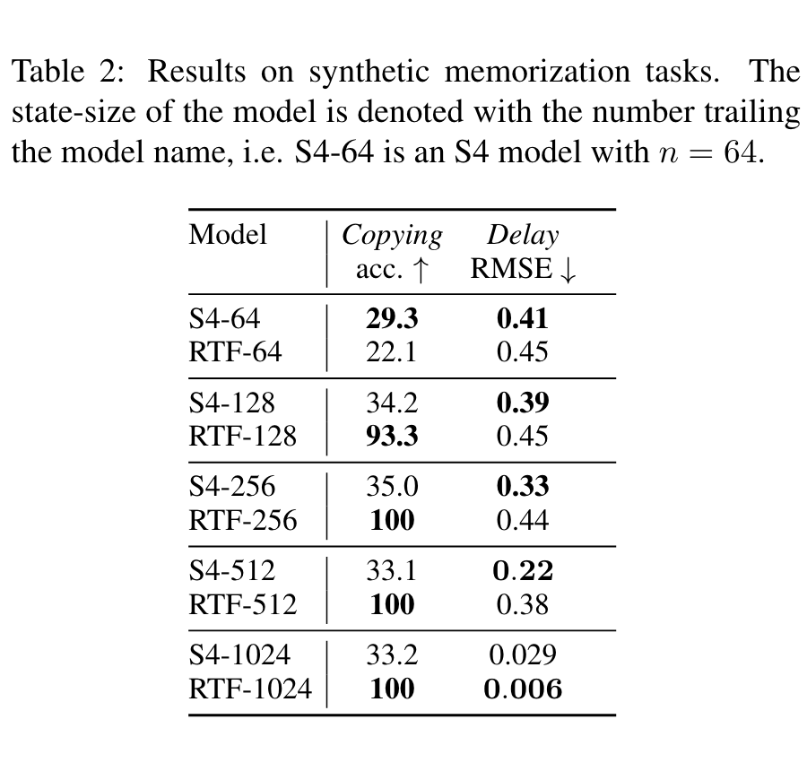
The first figure shows that RTF’s computational complexity (time and space) has no obvious relationship with the state size. Because of this, we can improve RTF’s performance by increasing the state size (since it doesn’t increase complexity), as shown in the second chart. Readers can refer to the original paper for other experimental results.

Summary

This article introduced RTF, a new work on SSM models. It observes that the generating function of the convolution kernel of a linear RNN can actually be expressed as a rational function (a fractional polynomial). Utilizing this feature, we can transfer all parameterization of the SSM to the generating function space and use the Discrete Fourier Transform for acceleration, significantly simplifying the entire calculation process. Compared with S4’s "diagonal + low-rank" decomposition, RTF is also more concise and intuitive.

Original address: https://kexue.fm/archives/10180