Private Reflections on Multimodal Ideas (Part 2): Autoregression

The Meaning of Lossless

First, let’s clarify the meaning of “lossless.” Lossless does not mean that there cannot be a single bit of loss throughout the entire calculation process. That is unrealistic and does not align with our understanding of the essence of deep learning. As mentioned in the 2015 article “Chatting: Neural Networks and Deep Learning”, the key to the success of deep learning is information loss. Therefore, the meaning of lossless here is simple: we hope that the input to the model is as lossless as possible.

The mainstream architecture of current multimodal models is still the Transformer. Many works first perform “pre-processing” on images before inputting them into the Transformer, such as simply dividing image pixels into patches, extracting features through a VAE, or discretizing them through VQ. Their common characteristic is transforming the image from a w \times h \times 3 array into an s \times t \times d array (where s < w, t < h), which we can collectively call generalized “Patchify.” Different Patchify methods may have different degrees of information loss. Among them, the information loss of VQ is often the most serious and explicit. For example, ByteDance’s recent TiTok compresses a 256 \times 256 image into 32 tokens. To understand its information loss, one doesn’t even need to calculate entropy, because its codebook size is only 4096. This means it can store at most 4096^{32} images. We know that there are more than 4096 Chinese characters; in other words, if there are 32 Chinese characters on an image, all permutations and combinations would exceed the upper limit of what this encoding method can express.

If an image has significant information loss before entering the model, it will inevitably limit the model’s image understanding capabilities. For instance, if TiTok’s 32 tokens are input into a model, it basically cannot perform OCR tasks. Moreover, this bottleneck of VQ is very fundamental; even changing it to 32 \times 32 tokens is unlikely to bring significant improvement unless the number of tokens reaches the order of magnitude of the original RGB pixels, but then the significance of VQ would be lost. Therefore, to better adapt to various image understanding tasks, the ideal image input method for multimodal models should be continuous features that are as lossless as possible, allowing the model itself to decide what to lose during the calculation process based on context.

Autoregressive Style

As mentioned at the beginning of this article, using continuous features as input is a very reasonable and natural way for image understanding. It only introduces extra difficulties for autoregressive (AR) image generation. Readers might wonder: why must images be generated autoregressively? Don’t we already have better generation methods like diffusion models?

First, we know that “autoregressive model + teacher forcing training” is a very universal learning approach, a typical manifestation of “hand-holding teaching,” so its potential is sufficient. Second, the example of diffusion models further illustrates the necessity of autoregression in image generation. Taking DDPM as an example, it is essentially an autoregressive model. In “Reflections on Generative Diffusion Models (2): DDPM = Autoregressive VAE”, we labeled it as autoregressive. It deconstructs a single image into a sequence x_T, x_{T-1}, \dots, x_1, x_0 and then models p(x_{t-1}|x_t). The training method is also essentially teacher forcing (so it also has the exposure bias problem). It can be said that DDPM is not only autoregressive but also the simplest 2-gram model among autoregressive models.

In fact, from early works like PixelRNN, PixelCNN, and NVAE, to today’s popular diffusion models and the practice of training language models by treating VQ-discretized images like text, the signal they convey is: For images, the question is not whether to do autoregression, but in what way to do it better. Its role is not only to empower multimodal models with image generation capabilities but also to serve as an important unsupervised learning pathway.

My idol Richard Feynman once said a famous quote: “What I cannot create, I do not understand.” This also holds true for large models; that is, “if you cannot generate, you cannot understand.” Of course, this statement might seem a bit arbitrary, as sufficient image understanding capabilities can seemingly be obtained through supervised learning of various image-text pairs. However, learning image understanding purely through supervised methods may have limited coverage on one hand, and is limited by the level of human understanding on the other. Therefore, we need unsupervised generative pre-training to obtain more comprehensive image understanding capabilities, which is consistent with the “Pretrain + SFT” pipeline of text.

Squared Error

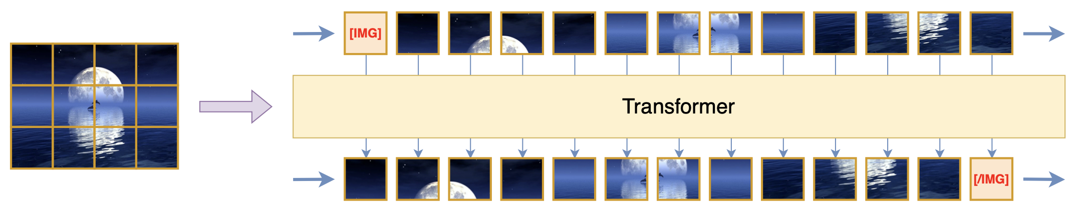
Some readers might think: after dividing the image into patches and sorting them, can’t we predict the next patch just like text? Even if the input format is changed from discrete to continuous features, wouldn’t we just need to replace the cross-entropy loss with squared error? It seems there is no difficulty in autoregressive learning for images? The logic seems sound, but in fact, the two key points mentioned here—Patchify sorting and the loss function—are both difficult problems to solve.

In this section, we first look at the loss function problem. Assuming the image has been divided into patches and sorted in some way, the image becomes a one-dimensional sequence of patches. Autoregressive learning is indeed the prediction of the next patch, as shown in the figure below:

However, the loss function here cannot simply be squared error (MSE, or equivalently, Euclidean distance, L2 distance). This is because the assumption about the distribution behind squared error is a Gaussian distribution: \begin{equation} \frac{1}{2\sigma^2}\Vert x_t - f(x_{< t})\Vert^2 = -\log \mathcal{N}(x_t;f(x_{< t}),\sigma^2) + \text{constant depending only on } \sigma \end{equation} That is, the negative log-likelihood of the Gaussian distribution \mathcal{N}(x_t;f(x_{< t}),\sigma^2) is exactly the squared error (where \sigma is a constant). This means that using squared error assumes p(x_t|x_{< t}) is \mathcal{N}(x_t;f(x_{< t}),\sigma^2). But if we think carefully, we find that this assumption is far from reality. If it were true, then sampling x_t could be done via x_t = f(x_{< t}) + \sigma\varepsilon, where \varepsilon is noise from a standard Gaussian distribution. Then x_t would inevitably have many noisy points, which is clearly not always the case in reality.

Some readers might argue: why must we understand it from the perspective of probabilistic likelihood? Can’t I just understand it purely as a regression fitting problem? Probably not. Understanding it from a probabilistic perspective mainly involves two considerations: first, generative modeling eventually faces sampling, and writing out the probability distribution is necessary to construct a sampling method; second, even from a pure regression perspective, we need to justify the rationality of squared error, because there are many other losses we could use, such as L1 distance (MAE), Hinge Loss, etc. These losses are not equivalent to each other, nor are they entirely reasonable (in fact, none of these losses are reasonable because they are metrics defined from a purely mathematical perspective and do not perfectly align with human visual perception).

The Magic of Noise

Since the nature of the input image features determines the irrationality of squared error, the only way to solve this problem is to modify the input format of the image so that its corresponding conditional distribution better fits a Gaussian distribution. Currently, there are two specific schemes to refer to.

The first scheme is to encode images through a pre-trained Encoder, where regularization terms like the KL divergence of VAE are usually added during training to reduce variance. To put it more intuitively, features are compressed near a sphere (refer to “An Attempt to Understand VAE from a Geometric Perspective”). Using these features as image inputs makes the assumption that p(x_t|x_{< t}) is a Gaussian distribution more reasonable, so we can use squared error for autoregressive training. After training, we also need to train a separate Decoder to decode the sampled image features back into an image. This is roughly the scheme adopted by Emu2. The disadvantage is that the pipeline seems too long and not end-to-end enough.

The second scheme might surprise many people: adding noise. This is my own “behind closed doors” idea. We just said that if p(x_t|x_{< t}) were truly a Gaussian distribution, then intuitively x_t should have many noisy points, but in reality, it doesn’t. To satisfy this condition, why don’t we just add some noise ourselves? Adding noise might not make p(x_t|x_{< t}) a perfect Gaussian distribution, but it can make it closer, especially when we add noise progressively, as shown below:

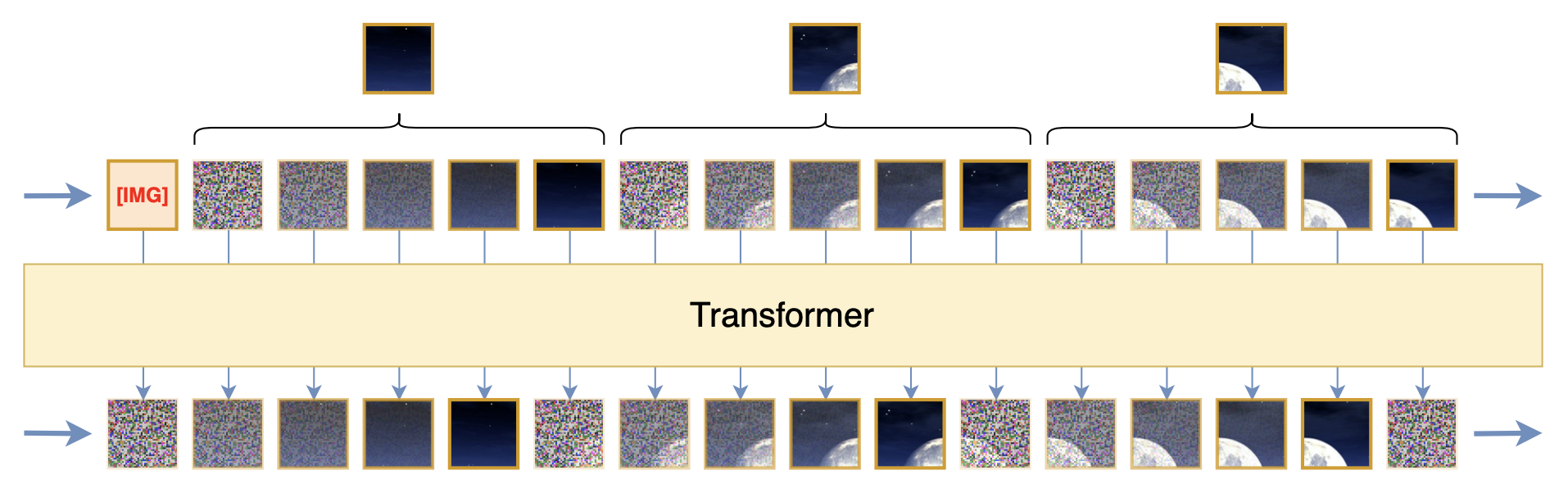
Readers familiar with diffusion models will easily realize that constructing a gradual sequence through noise addition and then training a recursive denoising model with squared error loss is exactly what a diffusion model does. Indeed, the core idea of the diffusion model is to make squared error a reasonable loss function through progressive noise addition, and the above scheme borrows this idea. Of course, the differences from conventional diffusion models are also obvious: for example, diffusion models add noise to the entire image, while here noise is added to patches; diffusion models model p(x_t|x_{t-1}), while here we model p(x_t|x_{< t}), and so on. In its final form, what is proposed here is a scheme that combines diffusion models for autoregressive learning of images.

Efficiency Issues

Extending the sequence through noise addition to make naive squared error usable, thereby making image autoregressive learning basically consistent with our initial conception (with just one extra step of noise addition), is undoubtedly a very comfortable result. However, things are not so optimistic. This scheme has at least two major problems, which can be summarized by one word—efficiency.

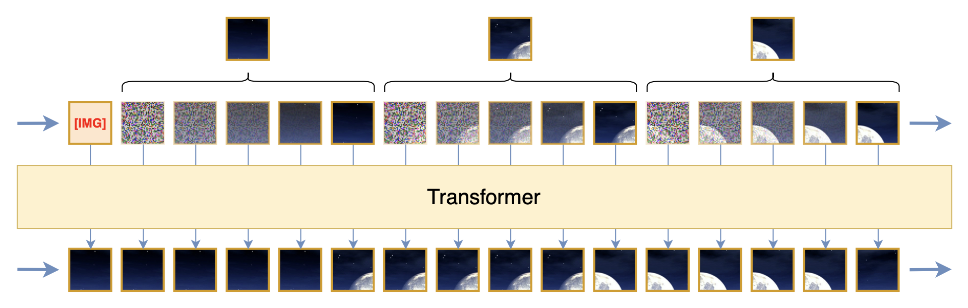
First is the learning efficiency problem. We discussed this in the first article introducing diffusion models, “Reflections on Generative Diffusion Models (1): DDPM = Demolition + Construction”. The general idea is that this training objective of predicting the noisy image at time t from the noisy image at time t-1 requires double sampling of noise, which leads to larger training variance. Therefore, more training steps are needed to reduce this variance. After a series of variance reduction techniques, we find that a more efficient way is to directly predict the original image (or equivalently, predict the difference between it and the original image):

Some readers might not understand: didn’t we just say that the original image has no noise and doesn’t fit a Gaussian distribution, so squared error cannot be used as a loss? This problem is indeed not easy to explain intuitively; we can understand it as a coincidence of the Gaussian distribution. In this case, squared error is still usable. For a more standard explanation, please refer to Part 3 and Part 4 of the diffusion model series.

Second is the computational efficiency problem. This is easy to understand. If each patch becomes T patches through noise addition, the sequence length becomes T times the original. Consequently, both training and inference costs will increase significantly. Furthermore, theoretically, noisy patches do not substantially help with image understanding; keeping only the clean, noise-free patch should, in principle, achieve the same effect. In other words, this scheme contains a large amount of redundant input and computation for image understanding.

There are also two ideas to solve this problem, which we will introduce one by one.

Separated Diffusion

If we are restricted to solving this within a single Transformer, we can consider adding a mask to the Attention. This includes two parts: 1. Diffusion theory and practice tell us that to predict x_t, x_{t-1} is sufficient, and earlier inputs can be ignored, meaning different noisy versions of the same patch do not need to attend to each other; 2. To reduce redundancy, for predictions between different patches and subsequent text tokens, we only need to attend to the clean patches. This forms an Attention Mask roughly as follows:

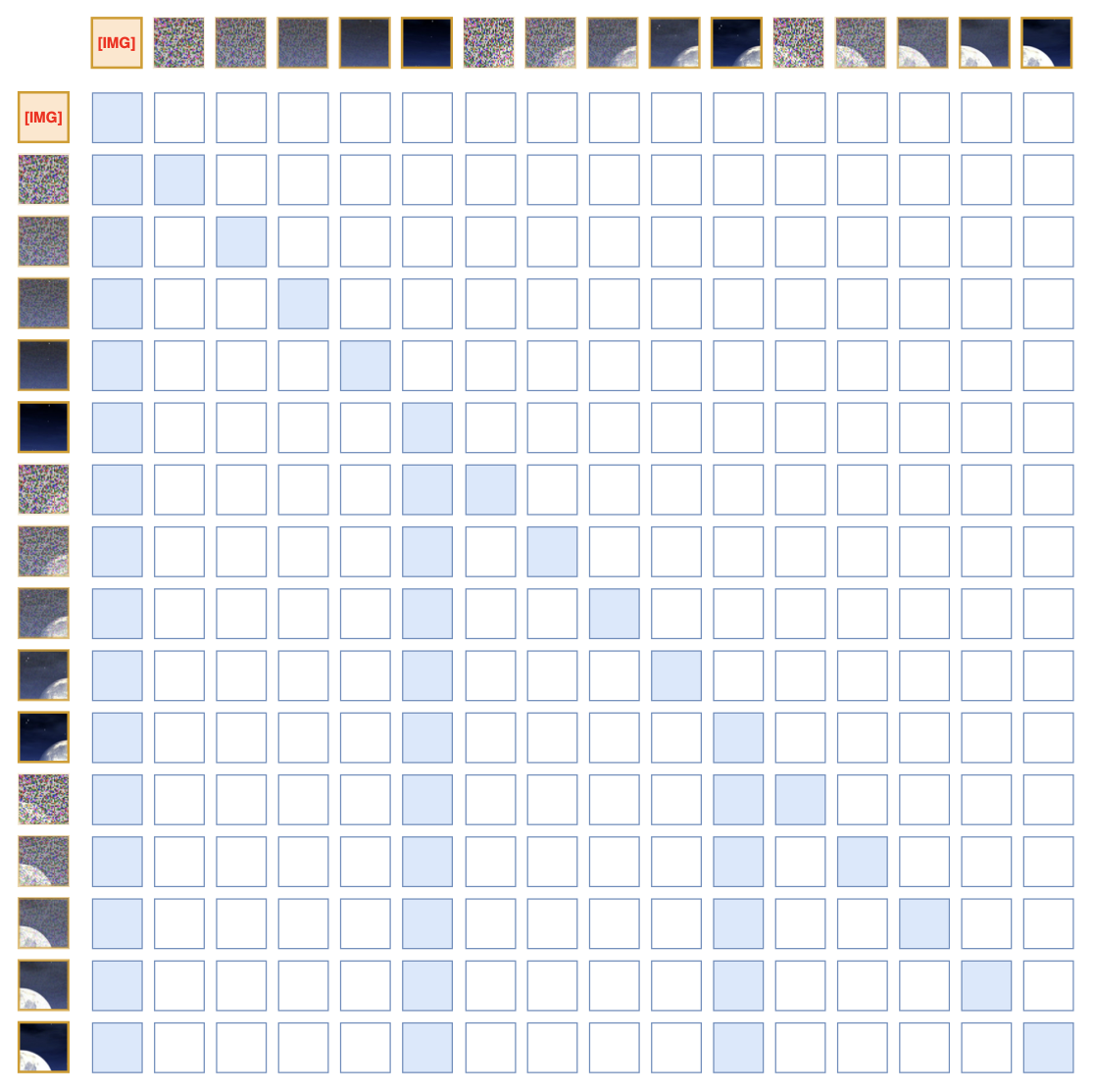
Since this Attention Mask has a fixed sparse pattern, it has significant potential for speedup. Moreover, because the attention of noisy patches is independent, we don’t have to include all T-1 noisy patches at once during training; we can just sample a portion for calculation each time. Of course, this is only a prototype; in practice, some details need careful consideration, such as the fact that noisy patches have almost no correlation, so their positional encodings need to be designed separately, etc. We won’t expand on that here.

If we allow two different models to be connected in series (but still trainable end-to-end), we can also separate the diffusion model. The Transformer only handles noise-free patches, and the output of the Transformer serves as the condition for the diffusion model, as shown below:

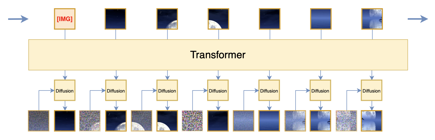
This is roughly the scheme proposed in Kaiming He’s new work “Autoregressive Image Generation without Vector Quantization”, though it was proposed even earlier in “Denoising Autoregressive Representation Learning”. Its advantage is that it makes the Transformer part more pure and elegant while also saving computation, because: 1) the separate diffusion model can be made smaller; 2) the diffusion part can follow conventional training strategies, sampling only one noise step per calculation. From the perspective of the loss function, it uses an additional diffusion model as the loss for predicting the next patch, thereby solving the shortcomings of squared error.

Generation Direction

Earlier, we mentioned that the two key points of image autoregressive learning are “Patchify sorting” and the “loss function.” We have just spent four sections barely smoothing out the loss function part, but that is only touching the threshold. Next, we will find a more pessimistic result—for the problem of “Patchify sorting,” we can hardly even find the threshold.

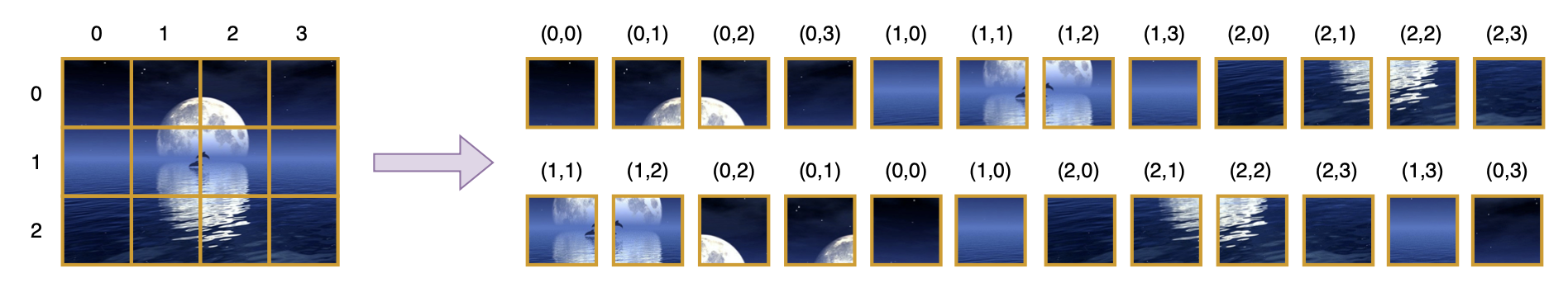
From the ultimate goal, “Patchify sorting” is to establish a generation sequence and direction for autoregressive learning. It consists of two steps: “Patchify” and “sorting.” “Patchify” in a narrow sense is a simple deformation and transposition of the pixel array: transforming a w \times h \times 3 array into s \times (w/s) \times t \times (h/t) \times 3, then transposing it to s \times t \times (w/s) \times (h/t) \times 3, and finally into s \times t \times (3wh/st). But in a broad sense, Patchify can refer to any scheme that transforms an image from a w \times h \times 3 array into an s \times t \times d array (where s < w, t < h), such as Stable Diffusion’s Encoder encoding images into Latents, or various VQ-Tokenizers turning images into discrete IDs.

“Sorting” is easier to understand. We know that images have two directions (dimensions): “length” and “width.” Most Patchify methods’ output features still retain this two-dimensional nature, while autoregressive generation is unidirectional, so a generation order must be specified. Common orders include 1) left-to-right then top-to-bottom, 2) spiral from center to edges, 3) Z-order starting from the top-left corner, etc. These sorting designs have a long history, dating back to the first generation of image autoregressive models that operated directly on pixels, such as PixelRNN/PixelCNN.

In general, “Patchify sorting” is the process of deconstructing an image into a one-dimensional sequence available for autoregressive learning. More simply, it is the conversion of an image from a two-dimensional sequence to a one-dimensional sequence. From the broadest perspective, the sequences of noisy images with different noise intensities constructed by diffusion models, as well as the sequences composed of multiple scales in “Visual Autoregressive Modeling: Scalable Image Generation via Next-Scale Prediction”, can all be included in this category. So, now that we have mentioned multiple schemes for deconstructing images, the natural question is: which scheme is better? What is the basis for judgment?

World Model

To answer this question, we first need to understand what the fundamental difficulty of visual generation is. In the first part of this series, we briefly mentioned that the difficulty of image generation lies in the difficulty of continuous probabilistic modeling. But in fact, this is a very superficial judgment. If it were only that, the situation would be much more optimistic, as we have already developed many continuous generative models like diffusion models. In reality, the difficulty is much more profound than we imagine...

The images we speak of can generally be divided into human-created pictures and photographs taken by cameras. Since the popularization of cameras and mobile phones, images on the internet are actually dominated by photographs. Therefore, image generation is basically equivalent to photograph generation. What is a photograph? It is a record of light, a projection of the three-dimensional world’s light onto a two-dimensional plane. And what is light? Light is an electromagnetic wave, and electromagnetic waves are solutions to Maxwell’s equations! From this reflection, we find an undeniable fact: A real natural photograph is essentially a solution to Maxwell’s equations. This means that perfect image generation inevitably touches upon the laws of physics—the origin of the world that many theoretical physicists tirelessly pursue!

Coincidentally, after the appearance of Sora, we often evaluate the quality of model-generated videos by whether they “conform to the physical laws of the real world.” In fact, seemingly simpler image generation can also have the evaluation dimension of “conforming to physical laws,” such as the distribution of light and shadow on the image. It’s just that with video, dynamics are added on top of optics (electromagnetism). Following this chain of thought, it becomes increasingly shocking or even terrifying, because it is equivalent to saying that a perfect visual generation model is actually numerically simulating various physical laws, or more exaggeratedly, it is simulating the evolution of the entire world and the entire universe. It is essentially a World Model. This is not just “hell-level” difficulty; it is “creation-level” difficulty.

Some readers might question: Maxwell’s equations are hard, but weren’t they discovered by humans? We have discovered even more difficult physical laws, such as quantum mechanics and general relativity, and are constantly approaching the ultimate law (Theory of Everything). So the difficulty of this matter doesn’t seem that high? No, let’s not be confused. Even if we can discover perfectly correct physical laws, that is a different matter from having the ability to “use these laws for numerical simulation.” For example, we can write down an equation but might not be able to solve it by hand. So, discovering physical laws does not mean we can use them to deduce or simulate the real world. More specifically, we can say here that the essence of a photograph is a solution to Maxwell’s equations, but no one can hand-draw a photograph.

(Note: The above series of reflections originated from the idea that “an image is essentially a solution to Maxwell’s equations,” which was shared with me by my leader, Zhou Xinyu, during a technical exchange. When I first heard this seemingly absurd but factually undeniable viewpoint, I was startled and shocked. Suddenly, I felt a sense of enlightenment regarding the fundamental difficulties of multimodal models.)

Human Values

In summary, the point this brainstorm wants to express is that a perfect visual generation model is a world model in the true sense, and its difficulty is of a creative magnitude. So, do we want to create a world? Do we have the ability to create a world? I believe that within the foreseeable future, the answer is no. After all, that would mean a feeling of using human power to contend with the entire universe. So the key here is to give up the concept of “perfection,” just as humans cannot hand-draw a photograph, but this still does not prevent humans from painting, nor does it prevent humans from conveying information through hand-drawing. For another example, when we evaluate whether a model-generated video conforms to physical laws, we are not actually measuring the video’s trajectory and substituting it into physical formulas to judge; it is purely visual observation combined with our intuitive perception of physical laws.

Simply put, it can be lossy, as long as it is lossless with respect to human values. So what does this have to do with the “Patchify sorting” mentioned earlier? We said at the beginning that autoregressive learning is not only to empower the model with generation capabilities but also to serve as an unsupervised learning pathway to improve the model’s understanding (if you can’t generate, you can’t understand). If we had a model with truly infinite fitting capability (creative capability), then all “Patchify sorting” methods would be equivalent, because the exact joint distribution does not depend on the decomposition method of random variables. But unfortunately, we don’t, so we must make choices.

Note that we hope to promote understanding through learning generation, and this “understanding” must be aligned with human visual understanding; this is the purpose of our AI training. However, among the “Patchify sorting” methods listed earlier, none conform to the way humans visually understand. More directly, human understanding of images is not from left to right or top to bottom, nor is it from the center to the edges or in a Z-order. In fact, humans don’t even understand images in units of patches, nor in the way of gradually adding noise like Diffusion. If we use existing “Patchify sorting” schemes for autoregressive learning, we indeed have a chance to empower the model with visual generation capabilities within a certain range. However, because these image deconstruction methods essentially do not conform to human visual understanding patterns, it is difficult to believe that this autoregressive learning can promote the model’s visual understanding capabilities—more accurately, it is difficult to promote the model’s ability to imitate human visual understanding.

The main reason for this difficulty is that an image is a “result” and does not contain a “process.” Take human-created images as an example: whether hand-drawn or Photoshopped, the process is a step-by-step operation, but what is finally presented is an image that masks its creative process. This is different from text. Although we don’t know how an author conceived a passage, we know that most people write from left to right, so the text itself already contains its creation (writing) process. But what about a painting? Looking at a painting, do we know which part or which stroke the painter drew first? Obviously not. This is also why most people can write but cannot copy a painting. Thinking deeper, this can be understood as humans appearing to be better at imitating along the time dimension and not as good along the spatial dimension, because there is only one time dimension, while there are three spatial dimensions, and the latter has too much freedom.

Currently, it seems there is only one very “compromising” method to solve this problem: using as much image-text data as possible that conforms to human values (of course, other valuable supervisory signals for images can also be used) to supervisedly train a “Patchify sorting” model. Note that unlike common Vision Encoders, this model should directly output a one-dimensional sequence instead of retaining the two-dimensional nature of the image, thus eliminating the subsequent sorting step. For the model design, we can refer to TiTok (this is the third time we’ve mentioned TiTok); it essentially uses Cross Attention to convert two-dimensional sequences into one-dimensional sequences. Besides that, Q-Former can also achieve similar effects. In short, there won’t be much difficulty in model design; the core work becomes the data engineering of image-text pairs.

But in this case, it’s hard to say how far the model can go, because we originally hoped to promote the model’s understanding capability through autoregressive learning, but now autoregressive learning depends on an Encoder trained through understanding tasks. Ideally, these two models would promote each other and evolve together, but in an unideal case, the model’s capability would be limited by the quantity and quality of the supervised data used to train the Encoder, failing to form true unsupervised learning.

Summary

This article continued to “build a car behind closed doors” with some ideas about multimodal learning, mainly focusing on visual autoregressive learning. The general content is:

1. Autoregressive learning both empowers the model with generation capabilities and serves as an unsupervised learning pathway to promote understanding through generation;

2. For images, the question is not whether to do autoregression, but in what way to do it better;

3. When inputting images as continuous features, their autoregressive learning faces two major difficulties: Patchify sorting and the loss function;

4. The loss function cannot simply be squared error; instead, one can consider following up with a small diffusion model to predict the next patch;

5. “Patchify sorting” is the fundamental difficulty of image autoregressive learning, and its choice determines whether autoregressive learning can truly promote understanding;

6. Perfect image/visual generation inevitably establishes a connection with physical laws, thereby constituting a “world model”;

7. But world models are difficult to achieve, so choosing a “Patchify sorting” method that aligns with human values is particularly important;

8. Finally, it seems we can only “compromise” by obtaining a “Patchify sorting” model aligned with human values through supervised learning.

There may be many “extreme theories” and “fallacies” here; readers are asked to discern and be tolerant. The main purpose of writing down these reflections is to look back someday in the future and see how much of my initial ideas were feasible and how much were laughable.

Reprinting should include the original address: https://kexue.fm/archives/10197

For more details on reprinting, please refer to: Scientific Space FAQ