As is well known, the standard loss for classification tasks is Cross Entropy (equivalent to Maximum Likelihood Estimation, or MLE). It is characterized by its simplicity and efficiency, but in certain scenarios, it reveals issues such as deviation from evaluation metrics and overconfidence. Consequently, there have been many improvement works. Previously, we have introduced some of these, such as "Revisiting the Class Imbalance Problem: Comparison and Connection between Weight Adjustment and Customizing Loss Functions", "How to Train Your Accuracy?", and "A Simple Solution to Mitigate Overconfidence in Cross Entropy". Since the training of Large Language Models (LLMs) can also be understood as a token-by-token classification task with Cross Entropy as the default loss, these improvement works remain valuable in the era of LLMs.
In this article, we introduce a work titled "EMO: Earth Mover Distance Optimization for Auto-Regressive Language Modeling". It proposes a new improved loss function, EMO, based on the idea of optimal transport, claiming to significantly improve the fine-tuning effects of LLMs. What are the details? Let’s find out.
Probability Divergence
Assume p_i is the probability of the i-th category predicted by the model, where i=1,2,\cdots,n, and t is the target category. Then the Cross Entropy loss is: \mathcal{L} = - \log p_t If we represent the label t in the form of a one-hot distribution \tau (i.e., \tau_t=1, \tau_i=0 for i \neq t, i \in [1,n]), it can be rewritten as: \mathcal{L} = - \sum_i \tau_i \log p_i This form also applies to non-one-hot labels \tau (i.e., soft labels). It is equivalent to optimizing the KL divergence between \tau and p: KL(\tau \Vert p) = \sum_i \tau_i \log \frac{\tau_i}{p_i} = \textcolor{cyan}{\sum_i \tau_i \log \tau_i} - \sum_i \tau_i \log p_i When \tau is given, the first term on the far right is a constant, so it is equivalent to the Cross Entropy objective.
This result indicates that when we perform MLE, or use Cross Entropy as the loss, we are essentially minimizing the KL divergence between the target distribution and the predicted distribution. Since the general generalization of KL divergence is f-divergence (refer to "Introduction to f-GAN: The Production Workshop of GAN Models"), it is natural to think that switching to other f-divergences might have an improvement effect. In fact, many works have followed this line of thought, such as the method introduced in "A Simple Solution to Mitigate Overconfidence in Cross Entropy", where the starting point of the paper is the "Total Variation distance," which is also a type of f-divergence.
Optimal Transport
However, every f-divergence has its problems. When it comes to an ideal measure between probability distributions, the "Earth Mover’s Distance (EMD)" based on the idea of optimal transport stands out. Readers unfamiliar with this can refer to my previous post "From Wasserstein Distance and Duality Theory to WGAN".
Briefly, the Earth Mover’s Distance is defined as the optimal transport cost between two distributions: \mathcal{C}[p,\tau] = \inf_{\gamma \in \Pi[p,\tau]} \sum_{i,j} \gamma_{i,j} c_{i,j} Here, \gamma \in \Pi[p,\tau] means that \gamma is any joint distribution with p and \tau as marginal distributions. c_{i,j} is a pre-given cost function representing the "cost of transporting from i to j." The \inf denotes the infimum, meaning that the lowest transport cost is used as the measure of difference between p and \tau. Just as replacing the Vanilla GAN based on f-divergence with the Wasserstein GAN based on optimal transport leads to better convergence properties, we expect that replacing the classification loss function with the Wasserstein distance between two distributions will also lead to better results.
When \tau is a one-hot distribution, the target distribution is a single point t. In this case, optimality is irrelevant as there is only one transport plan: moving everything from p to the same point t. Thus, we have: \mathcal{C}[p,\tau] = \sum_i p_i c_{i,t} \label{eq:emo}
If \tau is a general soft label distribution, calculating \mathcal{C}[p,\tau] is a linear programming problem, which is complex to solve. Since the distribution defined by p_i \tau_j also belongs to \Pi[p,\tau], we have: \mathcal{C}[p,\tau] = \inf_{\gamma \in \Pi[p,\tau]} \sum_{i,j} \gamma_{i,j} c_{i,j} \leq \sum_{i,j} p_i \tau_j c_{i,j} This is an easily computable upper bound that can also serve as an optimization objective. Equation [eq:emo] corresponds to \tau_j = \delta_{j,t}, where \delta is the Kronecker delta function.
Cost Function
Now let’s return to the scenario the original paper is concerned with—LLM fine-tuning, including continued pre-training and fine-tuning for downstream tasks. As mentioned at the beginning of this article, LLM training can be understood as a token-by-token classification task (where categories are all tokens). Each label is one-hot, so Equation [eq:emo] applies.
Equation [eq:emo] still requires the cost function c_{i,t} to be defined. If we simply assume that as long as i \neq t, the cost is 1, i.e., c_{i,t} = 1 - \delta_{i,t}, then: \mathcal{C}[p,\tau] = \sum_i p_i c_{i,t} = \sum_i (p_i - p_i \delta_{i, t}) = 1 - p_t This is essentially maximizing a smooth approximation of accuracy (refer to "Notes on Function Smoothing: Differentiable Approximation of Non-differentiable Functions"). However, intuitively, giving the same degree of penalty to all i \neq t seems too simple. Ideally, different costs should be designed for each different i based on similarity—the greater the similarity, the lower the transport cost. Thus, we can design the transport cost as: c_{i,t} = 1 - \cos(\boldsymbol{e}_i, \boldsymbol{e}_t) = 1 - \left\langle \frac{\boldsymbol{e}_i}{\Vert\boldsymbol{e}_i\Vert}, \frac{\boldsymbol{e}_t}{\Vert\boldsymbol{e}_t\Vert} \right\rangle Here, \boldsymbol{e}_i, \boldsymbol{e}_t are pre-obtained Token Embeddings. The original paper uses the LM Head of the pre-trained model as the Token Embedding. Since the cost function must be pre-given according to the definition of optimal transport, the Token Embeddings used to calculate similarity must remain fixed during the training process.
With the cost function, we can calculate: \mathcal{C}[p,\tau] = \sum_i p_i c_{i,t} = \sum_i
\left(p_i - p_i \left\langle
\frac{\boldsymbol{e}_i}{\Vert\boldsymbol{e}_i\Vert},
\frac{\boldsymbol{e}_t}{\Vert\boldsymbol{e}_t\Vert} \right\rangle
\right) = 1 - \left\langle \sum_i p_i
\frac{\boldsymbol{e}_i}{\Vert\boldsymbol{e}_i\Vert},
\frac{\boldsymbol{e}_t}{\Vert\boldsymbol{e}_t\Vert} \right\rangle
This is the final training loss for EMO (Earth Mover Distance Optimization). Since
embedding_size is usually much smaller than
vocab_size, calculating \sum_i
p_i \frac{\boldsymbol{e}_i}{\Vert\boldsymbol{e}_i\Vert} first
significantly reduces the computational load.
Experimental Results
Since my research on LLMs is still in the pre-training stage and has not yet involved fine-tuning, I don’t have my own experimental results for now. We can only look at the experimental results from the original paper together. It must be said that the results in the original paper are quite impressive.
First, in the continued pre-training experiments on small models, the improvement over Cross Entropy (MLE) is as much as 10 points in some cases, achieving comprehensive SOTA:

It is worth mentioning that the evaluation metric used here is MAUVE, where larger is better. It was proposed in "MAUVE: Measuring the Gap Between Neural Text and Human Text using Divergence Frontiers" and is one of the automatic evaluation metrics most correlated with human judgment. Additionally, the TaiLr method used for comparison was briefly introduced in "A Simple Solution to Mitigate Overconfidence in Cross Entropy".
Some readers might wonder if EMO is better simply because the evaluation metric was chosen favorably. Not at all. Surprisingly, models trained with EMO even achieve better PPL (Perplexity), which is more closely related to MLE:
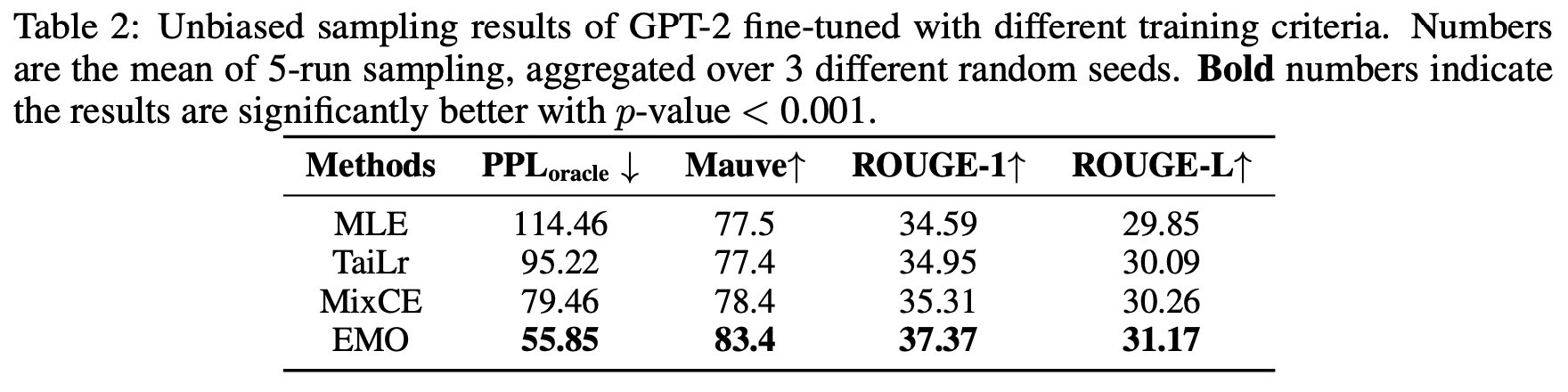
Then, the effect of fine-tuning LLAMA-7B/13B for downstream tasks in a few-shot setting is also excellent:

Finally, a comparison of different model scales and data scales shows that EMO performs well across various model and data sizes:

Personal Thinking
Overall, the "report card" of the original paper is very impressive and worth a try. The only concern might be that the experimental data volume in the original paper is not particularly large, and it is unclear whether the gap between EMO and MLE will narrow as the data volume increases further.
In my view, the reason EMO achieves better results is that it
calculates similarity through embeddings to assign more reasonable
losses to "synonyms," making the model’s learning more rational.
Although LLM training is formally a classification task, it is not a
simple right-or-wrong problem. It’s not the case that if the next
predicted token is different from the label token, the sentence is
necessarily unreasonable. Therefore, introducing semantic similarity to
design the loss is helpful for LLM training. It can be further
speculated that in cases where vocab_size is larger and
token granularity is coarser, the effect of EMO should be even better,
as a larger vocab_size might contain more "synonyms."
Of course, introducing semantic similarity also means that EMO is not suitable for training from scratch, as it requires a pre-trained LM Head as the Token Embedding. A possible solution could be to use other methods, such as the classic Word2Vec, to pre-train Token Embeddings. However, this might carry a risk: whether Token Embeddings trained in a classic way would lower the ceiling of LLM capabilities (due to inconsistency).
Furthermore, even if the Token Embedding is not an issue, using only EMO for training from scratch might lead to slow convergence. This is because, from the perspective of the loss function I proposed at the end of "How to Train Your Accuracy?":
First, find a smooth approximation of the evaluation metric, preferably expressed as an expected form for each sample. Then, pull the error in the wrong direction to infinity (to ensure the model focuses more on incorrect samples), while ensuring it is a first-order approximation of the original form in the correct direction.
In other words, to ensure convergence speed (when training from scratch), the loss in the wrong direction should ideally be pulled to infinity, which EMO clearly does not satisfy. Therefore, when using EMO for training from scratch, it would likely need to be a weighted combination of EMO and MLE to balance convergence speed and final performance.
Summary
This article introduced a new "substitute" for the Cross Entropy loss—EMO, based on the idea of optimal transport. Unlike previous minor improvements, EMO has achieved significant gains in LLM fine-tuning experiments.
When reposting, please include the original address: https://kexue.fm/archives/9797
For more details on reposting, please refer to: "Scientific Space FAQ"