Wasserstein distance (hereinafter referred to as "W-distance") is a distance function based on the idea of optimal transport to measure the degree of difference between two probability distributions. I have previously introduced it in blog posts such as "From Wasserstein Distance and Duality Theory to WGAN". For many readers, the first time they heard of W-distance was because of WGAN, which was released in 2017. It pioneered a new branch of understanding GANs from the perspective of optimal transport and elevated the status of optimal transport theory in machine learning. For a long time, GANs were the "main force" in the field of generative models, until the sudden emergence of diffusion models in the last two years, which caused GANs’ popularity to decline, though they remain powerful generative models in their own right.
Formally, the differences between diffusion models and GANs are quite obvious, so research on them has been relatively independent. However, a paper released at the end of last year, "Score-based Generative Modeling Secretly Minimizes the Wasserstein Distance", broke this barrier: it proved that the score matching loss of diffusion models can be written as an upper bound of the W-distance. This means that to some extent, minimizing the loss function of a diffusion model is, in fact, the same as WGAN—both are minimizing the W-distance between two distributions.
Analysis of the Conclusion
Specifically, the results of the original paper are directed at the SDE-style diffusion models introduced in "Generative Diffusion Models Part 5: SDE Perspective of the General Framework". Its core conclusion is the inequality (where I_t is a non-negative function of t; we will introduce its specific meaning in detail later): \mathcal{W}_2[p_0,q_0]\leq \int_0^T g_t^2 I_t \left(\mathbb{E}_{\boldsymbol{x}_t\sim p_t(\boldsymbol{x}_t)}\left[\left\Vert\nabla_{\boldsymbol{x}_t}\log p(\boldsymbol{x}_t) - \boldsymbol{s}_{\boldsymbol{\theta}}(\boldsymbol{x}_t,t)\right\Vert^2\right]\right)^{1/2}dt + I_T \mathcal{W}_2[p_T,q_T] \label{eq:w-neq} How should we understand this inequality? First, a diffusion model can be understood as a movement process of an SDE from t=T to t=0. p_T and q_T on the far right are the random sampling distributions at time T. p_T is usually a standard normal distribution, and in practical applications, we generally have q_T = p_T, so \mathcal{W}_2[p_T,q_T]=0. The reason the original paper explicitly writes it out is just to provide the most general theoretical result.
Next, p_0 on the left is the distribution of values at time t=0 obtained by solving the reverse SDE: d\boldsymbol{x}_t = \left[\boldsymbol{f}_t(\boldsymbol{x}_t) - g_t^2\nabla_{\boldsymbol{x}_t}\log p_t(\boldsymbol{x}_t) \right] dt + g_t d\boldsymbol{w} \label{eq:reverse-sde} starting from random points sampled from p_T. It is actually the data distribution to be generated. Meanwhile, q_0 is the distribution of values at time t=0 obtained by solving the SDE: d\boldsymbol{x}_t = \left[\boldsymbol{f}_t(\boldsymbol{x}_t) - g_t^2\boldsymbol{s}_{\boldsymbol{\theta}}(\boldsymbol{x}_t,t) \right] dt + g_t d\boldsymbol{w} starting from random points sampled from q_T, where \boldsymbol{s}_{\boldsymbol{\theta}}(\boldsymbol{x}_t,t) is the neural network approximation of \nabla_{\boldsymbol{x}_t}\log p_t(\boldsymbol{x}_t). Therefore, q_0 is actually the data distribution generated by the diffusion model. Thus, the meaning of \mathcal{W}_2[p_0,q_0] is the W-distance between the data distribution and the generated distribution.
Finally, the remaining integral term has a key part: \mathbb{E}_{\boldsymbol{x}_t\sim p_t(\boldsymbol{x}_t)}\left[\left\Vert\nabla_{\boldsymbol{x}_t}\log p(\boldsymbol{x}_t) - \boldsymbol{s}_{\boldsymbol{\theta}}(\boldsymbol{x}_t,t)\right\Vert^2\right] \label{eq:sm} This is exactly the "score matching" loss of the diffusion model. Therefore, when we use the score matching loss to train a diffusion model, we are actually indirectly minimizing the W-distance between the data distribution and the generated distribution. Unlike WGAN, which optimizes the \mathcal{W}_1[p_0,q_0] distance, here it is \mathcal{W}_2[p_0,q_0].
Note: To be precise, Equation [eq:sm] is not yet the loss function of the diffusion model. The loss function of the diffusion model should be "conditional score matching." The relationship between it and score matching is: \begin{aligned} &\,\mathbb{E}_{\boldsymbol{x}_t\sim p_t(\boldsymbol{x}_t)}\left[\left\Vert\nabla_{\boldsymbol{x}_t}\log p_t(\boldsymbol{x}_t) - \boldsymbol{s}_{\boldsymbol{\theta}}(\boldsymbol{x}_t,t)\right\Vert^2\right] \\ =&\, \mathbb{E}_{\boldsymbol{x}_t\sim p_t(\boldsymbol{x}_t)}\left[\left\Vert\mathbb{E}_{\boldsymbol{x}_0\sim p_t(\boldsymbol{x}_0|\boldsymbol{x}_t)}\left[\nabla_{\boldsymbol{x}_t}\log p_t(\boldsymbol{x}_t|\boldsymbol{x}_0)\right] - \boldsymbol{s}_{\boldsymbol{\theta}}(\boldsymbol{x}_t,t)\right\Vert^2\right] \\ \leq &\, \mathbb{E}_{\boldsymbol{x}_t\sim p_t(\boldsymbol{x}_t)}\mathbb{E}_{\boldsymbol{x}_0\sim p_t(\boldsymbol{x}_0|\boldsymbol{x}_t)}\left[\left\Vert\nabla_{\boldsymbol{x}_t}\log p_t(\boldsymbol{x}_t|\boldsymbol{x}_0) - \boldsymbol{s}_{\boldsymbol{\theta}}(\boldsymbol{x}_t,t)\right\Vert^2\right] \\ = &\, \mathbb{E}_{\boldsymbol{x}_0\sim p_0(\boldsymbol{x}_0),\boldsymbol{x}_t\sim p_t(\boldsymbol{x}_t|\boldsymbol{x}_0)}\left[\left\Vert\nabla_{\boldsymbol{x}_t}\log p_t(\boldsymbol{x}_t|\boldsymbol{x}_0) - \boldsymbol{s}_{\boldsymbol{\theta}}(\boldsymbol{x}_t,t)\right\Vert^2\right] \\ \end{aligned} The final result is the "conditional score matching" loss function of the diffusion model. The first equality is due to the identity \nabla_{\boldsymbol{x}_t}\log p_t(\boldsymbol{x}_t)=\mathbb{E}_{\boldsymbol{x}_0\sim p_t(\boldsymbol{x}_0|\boldsymbol{x}_t)}\left[\nabla_{\boldsymbol{x}_t}\log p_t(\boldsymbol{x}_t|\boldsymbol{x}_0)\right]. The second inequality is due to the generalization of the mean square inequality or Jensen’s inequality. The third equality is Bayes’ theorem. In other words, conditional score matching is an upper bound of score matching, and therefore also an upper bound of the W-distance.
From Equation [eq:w-neq], we can also simply understand why the objective function of the diffusion model discards the coefficient in front of the norm. Because the W-distance is a good measure of probability distributions, and g_t^2 I_t on the right side of Equation [eq:w-neq] is a monotonically increasing function of t, this means we should appropriately increase the score matching loss when t is small. In "Generative Diffusion Models Part 5: SDE Perspective", we derived the final form of score matching as: \frac{1}{\bar{\beta}_t^2}\mathbb{E}_{\boldsymbol{x}_0\sim \tilde{p}(\boldsymbol{x}_0),\boldsymbol{\varepsilon}\sim\mathcal{N}(\boldsymbol{0},\boldsymbol{I})}\left[\left\Vert \boldsymbol{\epsilon}_{\boldsymbol{\theta}}(\bar{\alpha}_t\boldsymbol{x}_0 + \bar{\beta}_t\boldsymbol{\varepsilon}, t) - \boldsymbol{\varepsilon}\right\Vert^2\right] Discarding the coefficient \frac{1}{\bar{\beta}_t^2} is equivalent to multiplying by \bar{\beta}_t^2, and \bar{\beta}_t^2 is also a monotonically increasing function of t. That is to say, one can simply consider that discarding the coefficient makes the training objective closer to the W-distance between the two distributions.
Preparation
Although the original paper provides the proof process for inequality [eq:w-neq], it involves a significant amount of knowledge related to optimal transport, such as continuity equations and gradient flows. In particular, a theorem it cites without proof is located in Chapter 8 of a monograph on gradient flows or Chapter 5 of another monograph on optimal transport, which makes the reading difficulty too high for me. After some attempts, I finally completed my own proof of (part of) inequality [eq:w-neq] last week. It only requires the definition of W-distance, basic differential equations, and the Cauchy-Schwarz inequality. Compared to the original paper’s proof, the difficulty of understanding should be significantly reduced. After several days of refinement, the proof process is as follows.
Before starting the proof, let’s prepare by organizing some basic concepts and conclusions that will be used. First is the W-distance, defined as: \mathcal{W}_{\rho}[p,q]=\left(\inf_{\gamma\in \Pi[p,q]} \iint \gamma(\boldsymbol{x},\boldsymbol{y}) \Vert\boldsymbol{x} - \boldsymbol{y}\Vert^{\rho} d\boldsymbol{x}d\boldsymbol{y}\right)^{1/\rho} where \Pi[p,q] refers to all joint probability density functions with p and q as marginal distributions, which describes a specific transport plan. This article only considers \rho=2, as only this case is convenient for subsequent derivation. Note that the definition of W-distance includes an infimum operation \inf, which means that for any \gamma\in \Pi[p,q] we can write down, we have: \mathcal{W}_2[p,q]\leq\left(\iint \gamma(\boldsymbol{x},\boldsymbol{y}) \Vert\boldsymbol{x} - \boldsymbol{y}\Vert^{2} d\boldsymbol{x}d\boldsymbol{y}\right)^{1/2} \label{eq:core-neq} This is the core idea of the proof I provide. The relaxation in the proof process mainly uses the Cauchy-Schwarz inequality: \begin{aligned} &\text{Vector version:}\quad\boldsymbol{x}\cdot\boldsymbol{y}\leq \Vert \boldsymbol{x}\Vert \Vert\boldsymbol{y}\Vert\\ &\text{Expectation version:}\quad\mathbb{E}_{\boldsymbol{x}}\left[f(\boldsymbol{x})g(\boldsymbol{x})\right]\leq \left(\mathbb{E}_{\boldsymbol{x}}\left[f^2(\boldsymbol{x})\right]\right)^{1/2}\left(\mathbb{E}_{\boldsymbol{x}}\left[g^2(\boldsymbol{x})\right]\right)^{1/2} \end{aligned} In the proof process, we assume that the function \boldsymbol{g}_t(\boldsymbol{x}) satisfies the "one-sided Lipschitz constraint," defined as: (\boldsymbol{g}_t(\boldsymbol{x}) - \boldsymbol{g}_t(\boldsymbol{y}))\cdot(\boldsymbol{x} - \boldsymbol{y}) \leq L_t \Vert \boldsymbol{x} - \boldsymbol{y}\Vert^2 \label{eq:assum} It can be proven that this is weaker than the common Lipschitz constraint (refer to "Lipschitz Constraint in Deep Learning: Generalization and Generative Models"), meaning that if a function \boldsymbol{g}_t(\boldsymbol{x}) satisfies the Lipschitz constraint, it must satisfy the one-sided Lipschitz constraint.
A Simple Trial
Inequality [eq:w-neq] is too general. Attempting to analyze the generalized result right away is not conducive to our thinking and understanding. Therefore, let’s simplify the problem first to see if we can prove a slightly weaker result. How to simplify? First, inequality [eq:w-neq] considers the difference in the initial distribution (note: the diffusion model is an evolution process from t=T to t=0, so t=T is the initial time and t=0 is the terminal time). Here, we first consider the same initial distribution. Additionally, the original reverse equation [eq:reverse-sde] is an SDE; here, we first consider a deterministic ODE.
Specifically, we consider starting from the same distribution q(\boldsymbol{z}) and sampling \boldsymbol{z} as the initial value at time T, then evolving along two different ODEs: \frac{d\boldsymbol{x}_t}{dt} = \boldsymbol{f}_t(\boldsymbol{x}_t),\quad \frac{d\boldsymbol{y}_t}{dt} = \boldsymbol{g}_t(\boldsymbol{y}_t) Let the distribution of \boldsymbol{x}_t at time t be p_t and the distribution of \boldsymbol{y}_t be q_t. We attempt to estimate an upper bound for \mathcal{W}_2[p_0,q_0].
We know that \boldsymbol{x}_t and \boldsymbol{y}_t both evolve from the same initial value \boldsymbol{z} through their respective ODEs, so they are actually deterministic functions of \boldsymbol{z}. More accurate notation would be \boldsymbol{x}_t(\boldsymbol{z}) and \boldsymbol{y}_t(\boldsymbol{z}); for simplicity, we omit \boldsymbol{z}. This means that the mapping \boldsymbol{x}_t \leftrightarrow \boldsymbol{y}_t corresponding to the same \boldsymbol{z} constitutes a correspondence (transport plan) between samples of p_t and q_t, as shown in the figure below:
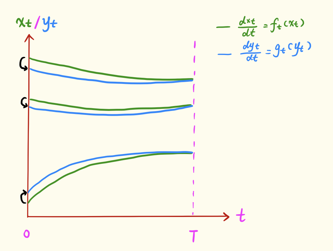
Thus, according to Equation [eq:core-neq], we can write: \mathcal{W}_2^2[p_t,q_t]\leq \mathbb{E}_{\boldsymbol{z}}\left[\Vert\boldsymbol{x}_t - \boldsymbol{y}_t\Vert^{2} \right]\triangleq \tilde{\mathcal{W}}_2^2[p_t,q_t] \label{eq:core-neq-2} Next, we relax \tilde{\mathcal{W}}_2^2[p_t,q_t]. To relate it to \boldsymbol{f}_t(\boldsymbol{x}_t) and \boldsymbol{g}_t(\boldsymbol{y}_t), we take its derivative: \begin{aligned} \pm\frac{d\left(\tilde{\mathcal{W}}_2^2[p_t,q_t]\right)}{dt}=&\, \pm2\mathbb{E}_{\boldsymbol{z}}\left[(\boldsymbol{x}_t - \boldsymbol{y}_t)\cdot \left(\frac{d\boldsymbol{x}_t}{dt} - \frac{d\boldsymbol{y}_t}{dt}\right)\right] \\ =&\, \pm 2\mathbb{E}_{\boldsymbol{z}}\left[(\boldsymbol{x}_t - \boldsymbol{y}_t)\cdot (\boldsymbol{f}_t(\boldsymbol{x}_t) - \boldsymbol{g}_t(\boldsymbol{y}_t))\right] \\ =&\, \pm 2\mathbb{E}_{\boldsymbol{z}}\left[(\boldsymbol{x}_t - \boldsymbol{y}_t)\cdot (\boldsymbol{f}_t(\boldsymbol{x}_t) - \boldsymbol{g}_t(\boldsymbol{x}_t))\right] \pm 2\mathbb{E}_{\boldsymbol{z}}\left[(\boldsymbol{x}_t - \boldsymbol{y}_t)\cdot (\boldsymbol{g}_t(\boldsymbol{x}_t) - \boldsymbol{g}_t(\boldsymbol{y}_t))\right] \\ \leq&\, 2\mathbb{E}_{\boldsymbol{z}}\left[\Vert\boldsymbol{x}_t - \boldsymbol{y}_t\Vert \Vert\boldsymbol{f}_t(\boldsymbol{x}_t) - \boldsymbol{g}_t(\boldsymbol{x}_t)\Vert\right] + 2\mathbb{E}_{\boldsymbol{z}}\left[L_t\Vert\boldsymbol{x}_t - \boldsymbol{y}_t\Vert^2\right] \\ \leq&\, 2\left(\mathbb{E}_{\boldsymbol{z}}\left[\Vert\boldsymbol{x}_t - \boldsymbol{y}_t\Vert^2\right]\right)^{1/2} \left(\mathbb{E}_{\boldsymbol{z}}\left[\Vert\boldsymbol{f}_t(\boldsymbol{x}_t) - \boldsymbol{g}_t(\boldsymbol{x}_t)\Vert^2\right]\right)^{1/2} + 2L_t\mathbb{E}_{\boldsymbol{z}}\left[\Vert\boldsymbol{x}_t - \boldsymbol{y}_t\Vert^2\right] \\ =&\, 2 \tilde{\mathcal{W}}_2[p_t,q_t] \left(\mathbb{E}_{\boldsymbol{z}}\left[\Vert\boldsymbol{f}_t(\boldsymbol{x}_t) - \boldsymbol{g}_t(\boldsymbol{x}_t)\Vert^2\right]\right)^{1/2} + 2L_t\tilde{\mathcal{W}}_2^2[p_t,q_t] \\ \end{aligned} \label{eq:der-neq-0} The first inequality uses the vector version of the Cauchy-Schwarz inequality and the one-sided Lipschitz constraint assumption [eq:assum]. The second inequality uses the expectation version of the Cauchy-Schwarz inequality. The \pm means that the resulting inequality holds regardless of whether we take + or -. The following derivation only uses the - side. Combining with (w^2)'=2ww', we get: -\frac{d\tilde{\mathcal{W}}_2[p_t,q_t]}{dt} \leq \left(\mathbb{E}_{\boldsymbol{z}}\left[\Vert\boldsymbol{f}_t(\boldsymbol{x}_t) - \boldsymbol{g}_t(\boldsymbol{x}_t)\Vert^2\right]\right)^{1/2} + L_t\tilde{\mathcal{W}}_2[p_t,q_t] \label{eq:der-neq-1} Using the method of variation of constants, let \tilde{\mathcal{W}}_2[p_t,q_t]=C_t \exp\left(\int_t^T L_s ds\right). Substituting this into the above equation gives: -\frac{dC_t}{dt} \leq \exp\left(-\int_t^T L_s ds\right)\left(\mathbb{E}_{\boldsymbol{z}}\left[\Vert\boldsymbol{f}_t(\boldsymbol{x}_t) - \boldsymbol{g}_t(\boldsymbol{x}_t)\Vert^2\right]\right)^{1/2} \label{eq:der-neq-2} Integrating both sides over [0,T] and combining with C_T=0 (since the two distributions are equal at the initial time, the distance is 0), we get: C_0 \leq \int_0^T \exp\left(-\int_t^T L_s ds\right)\left(\mathbb{E}_{\boldsymbol{z}}\left[\Vert\boldsymbol{f}_t(\boldsymbol{x}_t) - \boldsymbol{g}_t(\boldsymbol{x}_t)\Vert^2\right]\right)^{1/2} dt Thus: \tilde{\mathcal{W}}_2[p_0,q_0] \leq C_0 \exp\left(\int_0^T L_s ds\right) =\int_0^T I_t\left(\mathbb{E}_{\boldsymbol{z}}\left[\Vert\boldsymbol{f}_t(\boldsymbol{x}_t) - \boldsymbol{g}_t(\boldsymbol{x}_t)\Vert^2\right]\right)^{1/2} dt where I_t = \exp\left(\int_0^t L_s ds\right). According to Equation [eq:core-neq-2], this is also an upper bound for \mathcal{W}_2[p_0,q_0]. Finally, since the expression for the expectation is only a function of \boldsymbol{x}_t, and \boldsymbol{x}_t is a deterministic function of \boldsymbol{z}, the expectation with respect to \boldsymbol{z} is equivalent to the expectation directly with respect to \boldsymbol{x}_t: \mathcal{W}_2[p_0,q_0] \leq\int_0^T I_t\left(\mathbb{E}_{\boldsymbol{x}_t\sim p_t(\boldsymbol{x}_t)}\left[\Vert\boldsymbol{f}_t(\boldsymbol{x}_t) - \boldsymbol{g}_t(\boldsymbol{x}_t)\Vert^2\right]\right)^{1/2} dt \label{eq:w-neq-0}
Pressing On
In fact, the simplified inequality [eq:w-neq-0] is not fundamentally different from the more general [eq:w-neq]. Its derivation process already contains the general idea for deriving the complete result. Below, we complete the remaining derivation.
First, we generalize inequality [eq:w-neq-0] to scenarios with different initial distributions. Suppose the two initial distributions are p_T(\boldsymbol{z}_1) and q_T(\boldsymbol{z}_2). We sample the initial value from p_T(\boldsymbol{z}_1) to evolve \boldsymbol{x}_t, and sample the initial value from q_T(\boldsymbol{z}_2) to evolve \boldsymbol{y}_t. Thus, \boldsymbol{x}_t and \boldsymbol{y}_t are functions of \boldsymbol{z}_1 and \boldsymbol{z}_2 respectively, rather than functions of the same \boldsymbol{z} as before. Therefore, we cannot directly construct a transport plan. So, we also need a correspondence (transport plan) between \boldsymbol{z}_1 and \boldsymbol{z}_2. We choose it to be an optimal transport plan \gamma^*(\boldsymbol{z}_1,\boldsymbol{z}_2) between p_T(\boldsymbol{z}_1) and q_T(\boldsymbol{z}_2). Thus, we can write a result similar to Equation [eq:core-neq-2]: \mathcal{W}_2^2[p_t,q_t]\leq \mathbb{E}_{\boldsymbol{z}_1,\boldsymbol{z}_2\sim \gamma^*(\boldsymbol{z}_1,\boldsymbol{z}_2)}\left[\Vert\boldsymbol{x}_t - \boldsymbol{y}_t\Vert^{2} \right]\triangleq \tilde{\mathcal{W}}_2^2[p_t,q_t] \label{eq:core-neq-3} Due to the consistency of the definition, the relaxation process [eq:der-neq-0] still holds, except that the expectation \mathbb{E}_{\boldsymbol{z}} is replaced by \mathbb{E}_{\boldsymbol{z}_1,\boldsymbol{z}_2}. Therefore, inequalities [eq:der-neq-1] and [eq:der-neq-2] also hold. The difference is that when integrating both sides of [eq:der-neq-2] over [0,T], we no longer have C_T = 0. Instead, according to the definition, we have C_T=\tilde{\mathcal{W}}_2[p_T,q_T]=\mathcal{W}_2[p_T,q_T]. So, the final result is: \mathcal{W}_2[p_0,q_0] \leq\int_0^T I_t\left(\mathbb{E}_{\boldsymbol{x}_t\sim p_t(\boldsymbol{x}_t)}\left[\Vert\boldsymbol{f}_t(\boldsymbol{x}_t) - \boldsymbol{g}_t(\boldsymbol{x}_t)\Vert^2\right]\right)^{1/2} dt + I_T \mathcal{W}_2[p_T,q_T] \label{eq:w-neq-1}
Finally, we return to the diffusion model. In "Generative Diffusion Models Part 6: ODE Perspective", we derived that the same forward diffusion process actually corresponds to a family of reverse processes: d\boldsymbol{x} = \left(\boldsymbol{f}_t(\boldsymbol{x}) - \frac{1}{2}(g_t^2 + \sigma_t^2)\nabla_{\boldsymbol{x}}\log p_t(\boldsymbol{x})\right) dt + \sigma_t d\boldsymbol{w} \label{eq:sde-reverse-2} where \sigma_t is a standard deviation function that can be freely chosen. When \sigma_t=g_t, it becomes Equation [eq:reverse-sde]. Since we analyzed ODEs above, let’s first consider the case where \sigma_t=0. In this case, the result [eq:w-neq-1] is still applicable, but we replace \boldsymbol{f}_t(\boldsymbol{x}_t) with \boldsymbol{f}_t(\boldsymbol{x}_t) - \frac{1}{2}g_t^2\nabla_{\boldsymbol{x}_t}\log p_t(\boldsymbol{x}_t) and \boldsymbol{g}_t(\boldsymbol{x}_t) with \boldsymbol{f}_t(\boldsymbol{x}_t) - \frac{1}{2}g_t^2\boldsymbol{s}_{\boldsymbol{\theta}}(\boldsymbol{x}_t,t). Substituting these into Equation [eq:w-neq-1] yields the conclusion [eq:w-neq] presented at the beginning of the article. Of course, don’t forget the one-sided Lipschitz constraint assumption [eq:assum] we made for \boldsymbol{g}_t(\boldsymbol{x}_t) during the derivation. Now we can make assumptions for \boldsymbol{f}_t(\boldsymbol{x}_t) and \boldsymbol{s}_{\boldsymbol{\theta}}(\boldsymbol{x}_t,t) respectively; these details will not be expanded upon.
A Difficult Conclusion
Following the procedure, we should continue to complete the final proof for \sigma_t\neq 0. However, unfortunately, the logic of this article cannot fully prove the SDE case. Below is my analysis process. In fact, for most readers, understanding the ODE example in the previous section is enough to glimpse the essence of Equation [eq:w-neq-1]. The complete details are not overly important.
For simplicity, let’s take [eq:reverse-sde] as an example. A more general [eq:sde-reverse-2] can be analyzed similarly. We need to estimate the difference in the evolution trajectory distributions of the following two SDEs: \left\{\begin{aligned} d\boldsymbol{x}_t =&\, \left[\boldsymbol{f}_t(\boldsymbol{x}_t) - g_t^2\nabla_{\boldsymbol{x}_t}\log p_t(\boldsymbol{x}_t) \right] dt + g_t d\boldsymbol{w}\\ d\boldsymbol{y}_t =&\, \left[\boldsymbol{f}_t(\boldsymbol{y}_t) - g_t^2\boldsymbol{s}_{\boldsymbol{\theta}}(\boldsymbol{y}_t,t) \right] dt + g_t d\boldsymbol{w} \end{aligned}\right. That is, how much the final distribution is affected by replacing the accurate \nabla_{\boldsymbol{x}_t}\log p_t(\boldsymbol{x}_t) with the approximate \boldsymbol{s}_{\boldsymbol{\theta}}(\boldsymbol{y}_t,t). My proof idea is also to transform it into an ODE and then use the previous proof process. First, according to Equation [eq:sde-reverse-2], we know the ODE corresponding to the first SDE is: \begin{aligned} d\boldsymbol{x}_t &= \left[\boldsymbol{f}_t(\boldsymbol{x}_t) - g_t^2\nabla_{\boldsymbol{x}_t}\log p_t(\boldsymbol{x}_t) \right] dt + g_t d\boldsymbol{w}\\ &\Downarrow \\ d\boldsymbol{x}_t &= \left[\boldsymbol{f}_t(\boldsymbol{x}_t) - \frac{1}{2}g_t^2\nabla_{\boldsymbol{x}_t}\log p_t(\boldsymbol{x}_t) \right] dt \end{aligned} As for the derivation of the ODE corresponding to the second SDE, it requires some skill. It first needs to be changed into the form of -g_t^2\nabla_{\boldsymbol{y}_t}\log q_t(\boldsymbol{y}_t), and then Equation [eq:sde-reverse-2] is used: \begin{aligned} d\boldsymbol{y}_t &= \left[\boldsymbol{f}_t(\boldsymbol{y}_t) - g_t^2\boldsymbol{s}_{\boldsymbol{\theta}}(\boldsymbol{y}_t,t) \right] dt + g_t d\boldsymbol{w} \\ &\Downarrow \\ d\boldsymbol{y}_t &= \Big[\underbrace{\boldsymbol{f}_t(\boldsymbol{y}_t) - g_t^2\boldsymbol{s}_{\boldsymbol{\theta}}(\boldsymbol{y}_t,t) + g_t^2\nabla_{\boldsymbol{y}_t}\log q_t(\boldsymbol{y}_t)}_{\text{treated as a whole}} - g_t^2\nabla_{\boldsymbol{y}_t}\log q_t(\boldsymbol{y}_t) \Big] dt + g_t d\boldsymbol{w} \\ &\Downarrow \\ d\boldsymbol{y}_t &= \left[\boldsymbol{f}_t(\boldsymbol{y}_t) - g_t^2\boldsymbol{s}_{\boldsymbol{\theta}}(\boldsymbol{y}_t,t) + g_t^2\nabla_{\boldsymbol{y}_t}\log q_t(\boldsymbol{y}_t) - \frac{1}{2}g_t^2\nabla_{\boldsymbol{y}_t}\log q_t(\boldsymbol{y}_t) \right] dt \\ &\Downarrow \\ d\boldsymbol{y}_t &= \left[\boldsymbol{f}_t(\boldsymbol{y}_t) - g_t^2\boldsymbol{s}_{\boldsymbol{\theta}}(\boldsymbol{y}_t,t) + \frac{1}{2}g_t^2\nabla_{\boldsymbol{y}_t}\log q_t(\boldsymbol{y}_t)\right] dt \end{aligned} Repeating the relaxation process [eq:der-neq-0] for these two ODEs (taking the negative sign for \pm), the main difference is an extra term: -\frac{1}{2}g_t^2\mathbb{E}_{\boldsymbol{z}}\left[(\boldsymbol{x}_t - \boldsymbol{y}_t)\cdot (\nabla_{\boldsymbol{x}_t}\log p_t(\boldsymbol{x}_t)-\nabla_{\boldsymbol{y}_t}\log q_t(\boldsymbol{y}_t))\right] If this term is less than or equal to 0, then the relaxation process [eq:der-neq-0] still holds, and all subsequent results also hold, with the final conclusion taking the same form as Equation [eq:w-neq-1].
So, the remaining question is whether we can prove: \mathbb{E}_{\boldsymbol{z}}\left[(\boldsymbol{x}_t - \boldsymbol{y}_t)\cdot (\nabla_{\boldsymbol{x}_t}\log p_t(\boldsymbol{x}_t)-\nabla_{\boldsymbol{y}_t}\log q_t(\boldsymbol{y}_t))\right]\geq 0 Unfortunately, counterexamples can be given to show that it generally does not hold. A similar term appeared in the proof process of the original paper, but the distribution for the expectation was not \boldsymbol{z}, but the optimal transport distribution of \boldsymbol{x}_t and \boldsymbol{y}_t. Under this premise, the original paper directly throws out conclusions from two references as lemmas and completes the proof in a few lines. It must be said that the authors of the original paper are very familiar with optimal transport content, "picking up" various literature conclusions with ease. It is just difficult for a novice reader like me; wanting to understand it thoroughly is hard, so I can only stop here.
In particular, we cannot make a one-sided Lipschitz constraint assumption for \nabla_{\boldsymbol{x}_t}\log p_t(\boldsymbol{x}_t) or \nabla_{\boldsymbol{y}_t}\log q_t(\boldsymbol{y}_t), because it is easy to find distributions whose log-gradients do not satisfy the one-sided Lipschitz constraint. Therefore, to prove this inequality, one can only refer to the original paper’s idea of using the properties of the distribution itself, without imposing additional assumptions.
Summary
This article introduces a new theoretical result showing that the score matching loss of diffusion models can be written as an upper bound of the W-distance, and provides a partial proof. This result means that, to some extent, diffusion models and WGAN share the same optimization goal—diffusion models are also secretly optimizing the W-distance!
Original article address: https://kexue.fm/archives/9467