The Road to Transformer Upgrade: 8. Length Extrapolation and Positional Robustness

Problem Analysis

In previous articles, we analyzed the reasons for length extrapolation and positioned it as "a problem of length inconsistency between training and prediction." Specifically, there are two points of inconsistency:

1. During prediction, positional encodings (whether absolute or relative) that were never seen during training are used;

2. During prediction, the number of tokens processed by the attention mechanism far exceeds the number during training.

Regarding point 2, more tokens lead to more dispersed attention (or an increase in the entropy of attention), resulting in training-prediction inconsistency. We previously discussed and preliminarily solved this in "Looking at the Scale Operation of Attention from Entropy Invariance". The solution is to modify the Attention from: \begin{equation} \text{Attention}(Q,K,V) = \text{softmax}\left(\frac{QK^{\top}}{\sqrt{d}}\right)V \end{equation} to: \begin{equation} \text{Attention}(Q,K,V) = \text{softmax}\left(\frac{\log_{m} n}{\sqrt{d}}QK^{\top}\right)V \end{equation} where m is the training length and n is the prediction length. With this modification (hereafter referred to as "\log n scaled attention"), the entropy of attention remains more stable as the length changes, alleviating this inconsistency. Personal experimental results show that, at least on MLM tasks, "\log n scaled attention" performs better in length extrapolation.

Therefore, we can consider point 2 of the inconsistency to be preliminarily resolved. Next, we should focus on solving point 1.

Randomized Positions

Point 1 of the inconsistency is that "unseen positional encodings are used during prediction." To solve this, one should "train the positional encodings used in prediction during the training phase." A paper from ACL22 (still in anonymous review at the time of the original post), "Randomized Positional Encodings Boost Length Generalization of Transformers", first considered the problem from this perspective and proposed a solution.

The idea of the paper is simple:

Randomized Position Training: Let N be the training length (N=40 in the paper) and M be the prediction length (M=500 in the paper). Select a larger L > M (a hyperparameter, L=2048 in the paper). During the training phase, the position sequence corresponding to a sequence of length N was originally [0, 1, \dots, N-2, N-1]. Now, it is changed to randomly selecting N non-repeating integers from \{0, 1, \dots, L-2, L-1\} and arranging them in ascending order as the position sequence for the current sequence.

Reference code based on numpy:

def random_position_ids(N, L=2048):
    """Randomly pick N non-repeating integers from [0, L) and sort them ascendingly.
    """
    return np.sort(np.random.permutation(L)[:N])

During the prediction phase, one can sample the position sequence randomly in the same way, or directly take points uniformly within the interval (personal experiments show that uniform sampling generally works better). This solves the problem of positional encodings not being trained during the prediction phase. It is not difficult to understand that this is a very simple training trick (hereafter referred to as "randomized position training"), aiming to make the Transformer more robust to the choice of positions. However, as we will see later, it achieves a significant improvement in length extrapolation. I also conducted experiments on the MLM task, and the results showed that it is effective for MLM as well, with the improvement being more pronounced when combined with "\log n scaled attention" (the original paper did not include the "\log n scaled attention" step).

A New Benchmark

Many related works, including the various Local Attention variants mentioned in the previous article, use language modeling tasks to construct evaluation metrics. However, whether it is unidirectional GPT or bidirectional MLM, they rely heavily on local information (locality). Therefore, previous solutions might have shown good extrapolation performance only because of the locality of language models. If switched to a non-local task, the effect might deteriorate. Perhaps because of this, the evaluation in this paper is not a conventional language model task, but rather a length generalization benchmark specifically proposed by Google last year in the paper "Neural Networks and the Chomsky Hierarchy" (hereafter referred to as the "CHE benchmark," i.e., "Chomsky Hierarchy Evaluation Benchmark"). This provides us with a new perspective for understanding length extrapolation.

This benchmark includes multiple tasks divided into three levels: R (Regular), DCF (Deterministic Context-Free), and CS (Context-Sensitive), with difficulty increasing at each level. A brief description of each task follows:

• Even Pairs (Difficulty R): Given a binary sequence, e.g., "aabba", determine if the total number of "ab" and "ba" 2-grams is even. In this example, the 2-grams are aa, ab, bb, ba; "ab" and "ba" appear twice in total, so the output is "Yes". This problem is also equivalent to determining if the first and last characters of the binary sequence are the same.

• Modular Arithmetic (Simple) (Difficulty R): Calculate the value of an expression consisting of five numbers \{0, 1, 2, 3, 4\} and three operators \{+, -, \times\}, and output the result modulo 5. For example, input 1 + 2 - 4 equals -1, which is 4 modulo 5, so output 4.

• Parity Check (Difficulty R): Given a binary sequence, e.g., "aaabba", determine if the number of "b"s is even. In this example, the number of "b"s is 2, so output "Yes".

• Cycle Navigation (Difficulty R): Given a ternary sequence where each element represents one of \{+0, +1, -1\}, output the final result of the operation starting from 0 modulo 5. For example, if 0, 1, 2 represent +0, +1, -1, then 010211 represents 0 + 0 + 1 + 0 - 1 + 1 + 1 = 2, so output 2 modulo 5.

• Modular Arithmetic (Difficulty DCF): Calculate the value of an expression consisting of \{0, 1, 2, 3, 4\}, parentheses (, ), and \{+, -, \times\}, and output the result modulo 5. For example, input -(1-2)\times(4-3\times(-2)) results in 10, which is 0 modulo 5, so output 0. Compared to the Simple version, this task adds "parentheses," making the calculation more complex.

• Reverse String (Difficulty DCF): Given a binary sequence, e.g., "aabba", output its reversed sequence "abbaa".

• Solve Equation (Difficulty DCF): Given an equation consisting of \{0, 1, 2, 3, 4\}, parentheses (, ), \{+, -, \times\}, and an unknown z, solve for z such that it holds modulo 5. For example, -(1-2)\times(4-z\times(-2))=0, then z=3. Although solving equations seems harder, since the equation is constructed by replacing a number in Modular Arithmetic with z, a solution is guaranteed to exist in \{0, 1, 2, 3, 4\}. Thus, it can theoretically be solved by enumeration combined with Modular Arithmetic, making its difficulty comparable to Modular Arithmetic.

• Stack Manipulation (Difficulty DCF): Given a binary sequence, e.g., "abbaa", and a sequence of stack operations consisting of "POP / PUSH a / PUSH b", e.g., "POP / PUSH a / POP", output the final stack result. In this example, output "abba".

• Binary Addition (Difficulty CS): Given two binary numbers, output their sum in binary. For example, input 10010 and 101, output 10111. Note that this needs to be trained and predicted at the character level rather than the numerical level, and the two numbers are provided serially rather than aligned in parallel (input as the string 10010+101).

• Binary Multiplication (Difficulty CS): Given two binary numbers, output their product in binary. For example, input 100 and 10110, output 1011000. Like Binary Addition, this is handled at the character level and provided serially (input as 100\times 10110).

• Compute Sqrt (Difficulty CS): Given a binary number, output the binary representation of the floor of its square root. For example, input 101001, output \lfloor\sqrt{101001}\rfloor=101. This difficulty is similar to Binary Multiplication, as one can enumerate from 0 to the given number.

• Duplicate String (Difficulty CS): Given a binary sequence, e.g., "abaab", output the sequence repeated once, "abaababaab". This simple-looking task is actually CS difficulty. Think about why.

• Missing Duplicate (Difficulty CS): Given a binary sequence with a missing value, e.g., "ab_aba", where the original complete sequence is known to be a duplicate sequence (as in the previous task), predict the missing value. In this example, output "a".

• Odds First (Difficulty CS): Given a binary sequence t_1 t_2 t_3 \dots t_n, output t_1 t_3 t_5 \dots t_2 t_4 t_6 \dots. For example, input "aaabaa", output "aaaaba".

• Bucket Sort (Difficulty CS): Given an n-element numerical sequence (where each number is one of n given numbers), return the sequence sorted in ascending order. For example, input 421302214 should output 011222344.

As can be seen, these tasks share a common characteristic: their operations have fixed simple rules, and theoretically, the inputs are of unlimited length. Thus, we can train on short sequences and test whether the training results on short sequences can generalize to long sequences. In other words, it serves as a very strong benchmark for length extrapolation.

Experimental Results

First, let’s introduce the experimental results of the original paper "Neural Networks and the Chomsky Hierarchy", which compared several RNN models and Transformer models (the evaluation metric is the average accuracy of characters, not the exact match rate of the whole result):

The results might be surprising: the "highly popular" Transformer has the worst length extrapolation effect (the Transformer here was tested with different positional encodings, taking the optimal value for each task). The best is Tape-RNN. The paper gives them the following ratings: \underbrace{\text{Transformer}}_{\text{R}^-} < \underbrace{\text{RNN}}_{\text{R}} < \underbrace{\text{LSTM}}_{\text{R}^+} < \underbrace{\text{Stack-RNN}}_{\text{DCF}} < \underbrace{\text{Tape-RNN}}_{\text{CS}}

The randomized position training method proposed in "Randomized Positional Encodings Boost Length Generalization of Transformers" recovers some ground for the Transformer:

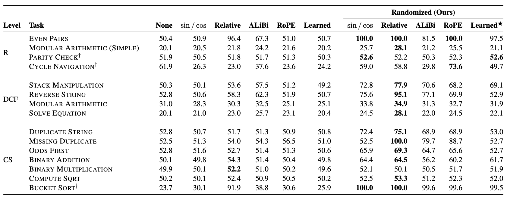
It can be seen that under randomized position training, Transformers with any positional encoding show significant improvements. This further validates the conclusion of the previous article that length extrapolation has little to do with the design of the positional encoding itself. Notably, randomized position training achieved 100% accuracy on the Bucket Sort task for the first time. Although overall performance is still lacking, it is a major step forward compared to previous results (I wonder if combining it with "\log n scaled attention" would help?). It is also worth noting that the table shows ALIBI, which performs well in language model tasks, does not show any advantage on the CHE benchmark. Especially after adding randomized position training, its average metric is worse than RoPE. This preliminarily confirms the previous guess that the good performance of various Local Attention variants is likely because the language model evaluation tasks themselves have strong locality; for the non-local CHE benchmark, these methods have no advantage.

Reflections on Principles

Upon reflection, "randomized position training" is quite puzzling. For simplicity, let L=2048, N=64, M=512. In this case, the average position sequence used in the training phase is roughly [0, 32, 64, \dots, 2016], while the average position sequence used in the prediction phase is [0, 4, 8, \dots, 2044]. The difference between adjacent positions is different in the training and prediction phases, which could also be called a kind of inconsistency. Yet, it still performs well. Why?

We can understand it from the perspective of "order." Since the position IDs in the training phase are randomly sampled, the difference between adjacent positions is also random. Therefore, whether using relative or absolute positions, it is unlikely that the model obtains positional information through precise position IDs. Instead, it receives a fuzzy positional signal—more accurately, it encodes position through the "order" of the position sequence rather than the position IDs themselves. For example, the position sequence [1, 3, 5] is equivalent to [2, 4, 8] because they are both sequences arranged in ascending order. Randomized position training "forces" the model to learn an equivalence class: all position sequences arranged in ascending order are equivalent and interchangeable. This is the true meaning of positional robustness.

However, my own experimental results on MLM show that learning this "equivalence class" is still somewhat difficult for the model. A more ideal method would be to still use randomized positions during training so that the positional encodings for the prediction phase are also trained, but the first part of the position sequence in the prediction phase should be consistent with the average result of the randomized positions. In the previous example, if the position sequence used in the prediction phase is [0, 4, 8, \dots, 2044], we would want the average result of the randomized positions in the training phase to be [0, 4, 8, \dots, 252] (i.e., the first N elements of the sequence [0, 4, 8, \dots, 2044]), rather than [0, 32, 64, \dots, 2016]. This would make the consistency between training and prediction tighter.

Extensions

Consequently, I considered the following idea:

Mean-Equivalent Randomized Position Training: Let n follow a distribution with a mean of N and a sampling space of [0, \infty). During training, randomly sample an n, and then uniformly take N points from [0, n] as the position sequence.

Reference code:

def random_position_ids(N):
    """First randomly sample n, then take N points uniformly from [0, n].
    """
    n = sample_from_xxx()
    return np.linspace(0, 1, N) * n

Note that the position sequence sampled this way consists of floating-point numbers. Therefore, it is not suitable for discrete trainable positional encodings, but only for functional positional encodings such as Sinusoidal or RoPE. Below, we assume only functional positional encodings are considered.

The biggest problem with this idea is how to choose a suitable sampling distribution. My first reaction was the Poisson distribution, but considering that both the mean and variance of the Poisson distribution are n, estimating by the "3\sigma rule," it can only extrapolate to a length of n+3\sqrt{n}, which is clearly too short. After selection and testing, I found two distributions to be more suitable: one is the Exponential distribution, whose mean and standard deviation are both n. Even by the "3\sigma rule," it can extrapolate to a length of 4n, which is a more ideal range (actually even longer). The other is the Beta distribution, defined on [0, 1]. We can treat the test length as 1, so the training length is N/M \in (0, 1). The Beta distribution has two parameters \alpha, \beta, with a mean of \frac{\alpha}{\alpha+\beta}. After ensuring the mean equals N/M, we still have an extra degree of freedom to control the probability near 1, which is suitable for scenarios where we want to further expand the extrapolation range.

My experimental results show that "Mean-Equivalent Randomized Position Training" combined with "\log n scaled attention" achieves the best extrapolation effect on the MLM task (training length 64, test length 512, sampling distribution is Exponential). Since I hadn’t worked with the CHE benchmark before, I couldn’t test it immediately, so I’ll have to leave that for a future opportunity.

Summary

This article explores the length extrapolation of Transformers from the perspective of positional robustness and introduces new schemes such as "randomized position training" to enhance length extrapolation. At the same time, we introduced the new "CHE benchmark." Compared to conventional language model tasks, it possesses stronger non-locality and can more effectively evaluate work related to length extrapolation. Under this benchmark, previous methods related to attention localization did not show particularly outstanding performance. In contrast, "randomized position training" was more effective. This reminds us that we should evaluate the effectiveness of related methods on a more comprehensive set of tasks, rather than being limited solely to language model tasks.

Reprinted from: https://kexue.fm/archives/9444