In recent days, a problem titled “Four Ducks in a Semicircle” has gone viral online:
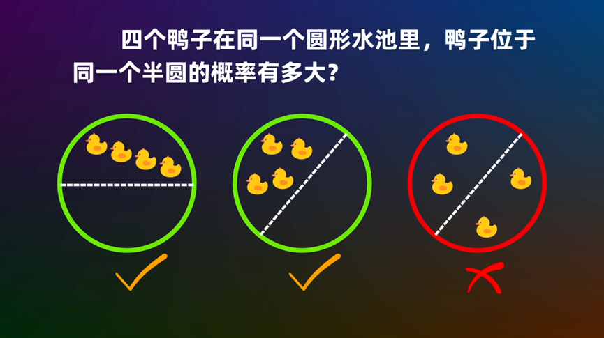
Many readers might have tried to solve it upon seeing it. Even Teacher Li Yongle dedicated a lecture to this problem (refer to “Four ducks in a circular pond, what is the probability they are in the same semicircle?”). Regarding the problem itself, the answer is not particularly difficult to calculate using various methods. What is slightly more challenging is its generalized version, as described in the title of this article: generalizing the number of ducks to n and the semicircle to a sector with a central angle \theta. Interestingly, when \theta \leq \pi, there is still a relatively elementary solution, but once \theta > \pi, the complexity begins to increase dramatically...
Problem Transformation
First, it should be clarified that we treat the ducks as points sampled from a uniform distribution within the circle. Generalizations such as the “physical area occupied by the ducks” will not be considered here. Regarding the “Four Ducks in a Semicircle” problem, it is easy to generalize it, for instance, to higher-dimensional spaces:
What is the probability that n points uniformly distributed within a d-dimensional hypersphere lie within the same d-dimensional hyper-hemisphere?
The answer to this generalization was provided in the paper “A Problem in Geometric Probability” published in 1962. Another generalization is the title of this article:
What is the probability that n points uniformly distributed within a circle lie within the same sector with a central angle \theta?
This article primarily discusses this problem. It can be equivalently transformed into (the reader is invited to think about how this transformation works):
If n points are chosen uniformly and randomly on the circumference of a circle, dividing the circumference into n arcs, what is the probability that the central angle subtended by the longest arc is greater than 2\pi - \theta?
Furthermore, it can be equivalently transformed into:
If n-1 points are chosen uniformly and randomly on a unit line segment, dividing the segment into n parts, what is the probability that the length of the longest segment is greater than 1 - \frac{\theta}{2\pi}?
Distribution Solution
In fact, the distribution involved in the last equivalent formulation has been well-discussed, for example, in the Zhihu question “What is the expected length of the longest segment when a (0, 1) interval is divided into n segments by random points?”. For the convenience of the reader, I will re-organize the explanation. The process is somewhat long, but it is necessary for finding a general solution (applicable for \theta > \pi).
It is worth noting that the extremum of multiple random variables belongs to the field of “Order Statistics,” which is common in machine learning. For example, the nearest neighbor estimation of entropy introduced in “EAE: Autoencoder + BN + Maximum Entropy = Generative Model” and the general construction of discrete distributions introduced in “Constructing Discrete Probability Distributions from a Reparameterization Perspective” can both be categorized as such.
Joint Distribution
Starting from the last equivalent formulation, let the unit line segment be divided by n-1 random points into n segments with lengths x_1, x_2, \dots, x_n from left to right (note: this just defines an order, they are not sorted by size). Let their joint probability density function be p_n(x_1, x_2, \dots, x_n). The answer in the Zhihu link is based directly on the fact that “p_n(x_1, x_2, \dots, x_n) is a uniform distribution.” However, I feel that the fact that “p_n(x_1, x_2, \dots, x_n) is a uniform distribution” is not immediately obvious, so I will derive it here.
First, note two facts:
x_1, x_2, \dots, x_n are subject to the constraint x_1 + x_2 + \dots + x_n = 1, so there are only n-1 degrees of freedom. We take the first n-1 variables as independent variables.
p_n(x_1, x_2, \dots, x_n) is a probability density, not a probability; p_n(x_1, x_2, \dots, x_n) dx_1 dx_2 \dots dx_{n-1} is the probability.
To understand why p_n(x_1, x_2, \dots, x_n) is a uniform distribution, we start with n=2. In this case, a single point is chosen uniformly in (0, 1) to divide the segment into two parts. Since the point is sampled from a uniform distribution (density is 1) and the point corresponds one-to-one with (x_1, x_2), we have p_2(x_1, x_2) = 1.
Next, consider n=3. The corresponding probability is p_3(x_1, x_2, x_3) dx_1 dx_2. There are two possibilities:
Sample one point first, dividing the segment into two parts (x_1, x_2 + x_3). The probability for this is p_2(x_1, x_2 + x_3) dx_1. Then sample another point to divide the x_2 + x_3 segment into (x_2, x_3). The probability for this part is dx_2. Multiplying them gives p_2(x_1, x_2 + x_3) dx_1 dx_2.
Sample one point first, dividing the segment into two parts (x_1 + x_2, x_3). The probability for this is p_2(x_1 + x_2, x_3) dx_2. Then sample another point to divide the x_1 + x_2 segment into (x_1, x_2). The probability for this part is dx_1. Multiplying them gives p_2(x_1 + x_2, x_3) dx_1 dx_2.
Adding them together: p_3(x_1, x_2, x_3) dx_1 dx_2 = p_2(x_1, x_2 + x_3) dx_1 dx_2 + p_2(x_1 + x_2, x_3) dx_1 dx_2 = 2 dx_1 dx_2 Thus p_3(x_1, x_2, x_3) = 2, which is also a uniform distribution. By induction, we can obtain: p_n(x_1, x_2, \dots, x_n) = (n - 1) p_{n-1}(x_1, x_2, \dots, x_{n-1}) = \dots = (n - 1)!
Marginal Distribution
With the joint distribution, we can find the marginal distribution for any k variables. This prepares us for using the “Inclusion-Exclusion Principle” in the next section. Since the joint distribution is uniform, the variables are symmetric. Therefore, without loss of generality, we can find the marginal distribution of the first k variables.
By definition: p_n(x_1, x_2, \dots, x_k) = \int \dots \int p_n(x_1, x_2, \dots, x_n) dx_{k+1} \dots dx_{n-1} Note the integration limits. The lower limit is naturally 0. Due to the constraint x_1 + x_2 + \dots + x_n = 1, the upper limit is different for each variable. Given x_1, x_2, \dots, x_i, the value of x_{i+1} can only range from 0 to 1 - (x_1 + x_2 + \dots + x_i). Thus, the precise form is: \int_0^{1 - (x_1 + \dots + x_k)} \dots \left[ \int_0^{1 - (x_1 + \dots + x_{n-2})} p_n(x_1, \dots, x_n) dx_{n-1} \right] \dots dx_{k+1} Since p_n(x_1, \dots, x_n) = (n-1)! is a constant, the above expression can be integrated sequentially. The final result is: p_n(x_1, x_2, \dots, x_k) = \frac{(n-1)!}{(n - k - 1)!} [1 - (x_1 + x_2 + \dots + x_k)]^{n-k-1} Now we can calculate the probability that x_1, x_2, \dots, x_k are each greater than given thresholds c_1, c_2, \dots, c_k (where c_1 + c_2 + \dots + c_k \leq 1): \begin{aligned} & P_n(x_1 > c_1, x_2 > c_2, \dots, x_k > c_k) = \int_{c_1}^{1 - (c_2 + \dots + c_k)} \dots \\ & \left[ \int_{c_{k-1}}^{1 - (x_1 + \dots + x_{k-2} + c_k)} \left[ \int_{c_k}^{1 - (x_1 + \dots + x_{k-1})} p_n(x_1, \dots, x_k) dx_k \right] dx_{k-1} \right] \dots dx_1 \end{aligned} The integration limits are derived similarly under the constraint \sum x_i = 1. Like p_n(x_1, \dots, x_n), this can be integrated sequentially, and the final result is surprisingly simple: P_n(x_1 > c_1, x_2 > c_2, \dots, x_k > c_k) = [1 - (c_1 + c_2 + \dots + c_k)]^{n-1}
Inclusion-Exclusion Principle
Now everything is ready for the “Inclusion-Exclusion Principle” to deliver the final blow. Recall that our goal is to find the probability of the longest segment length, i.e., for a threshold x, calculate P_n(\max(x_1, x_2, \dots, x_n) > x). The event \max(x_1, x_2, \dots, x_n) > x is the union of several events: \max(x_1, x_2, \dots, x_n) > x \quad \Leftrightarrow \quad x_1 > x \text{ \color{red}{or} } x_2 > x \text{ \color{red}{or} } \dots \text{ \color{red}{or} } x_n > x Crucially, when x < \frac{1}{2}, these events are not mutually exclusive. Therefore, we cannot simply sum the probabilities of each part; we must use the Inclusion-Exclusion Principle: \begin{aligned} P(\text{at least one } x_i > x) = & \sum P(\text{any one } x_i > x) \\ & \color{red}{-} \sum P(\text{any two } x_i, x_j > x) \\ & \color{red}{+} \sum P(\text{any three } x_i, x_j, x_l > x) \\ & \color{red}{-} \dots \end{aligned} According to the results of the previous section, the probability that any k chosen points are each greater than x is (1-kx)^{n-1}, and the number of ways to choose k points is \binom{n}{k}. Substituting these into the formula gives: \begin{aligned} P_n(\max(x_1, x_2, \dots, x_n) > x) &= \sum_{k=1, 1 - kx > 0}^n (-1)^{k-1} \binom{n}{k} (1-kx)^{n-1} \\ &= \binom{n}{1} (1 - x)^{n-1} - \binom{n}{2} (1 - 2x)^{n-1} + \dots \end{aligned}
Answer Analysis
For the problem at the beginning of this article, where x = 1 - \frac{\theta}{2\pi}, when x > \frac{1}{2} (i.e., \theta < \pi), the subsequent terms 1 - kx are all less than 0, meaning they do not exist in the summation. Thus, the answer is at its simplest: \binom{n}{1} (1 - x)^{n-1} = n \left(\frac{\theta}{2\pi}\right)^{n-1} When x < \frac{1}{2}, terms are added or subtracted depending on the specific value of x. The smaller x is, the more terms there are. This is what Teacher Li Yongle meant when he said, “When \theta is greater than 180 degrees, the situation becomes very complex.”
We can also find its expectation, which is the problem discussed in the Zhihu question. There is another interesting case: clearly, when x < \frac{1}{n}, we always have 1 - kx > 0, meaning all terms are used: P_n(\max(x_1, x_2, \dots, x_n) > x) = \sum_{k=1}^n (-1)^{k-1} \binom{n}{k} (1-kx)^{n-1} However, according to the “Pigeonhole Principle,” when a unit segment is divided into n parts, the length of the longest part must be at least \frac{1}{n}. This means P_n(\max(x_1, x_2, \dots, x_n) > \frac{1}{n}) = 1. Therefore, when x < \frac{1}{n}, it must hold that: \sum_{k=1}^n (-1)^{k-1} \binom{n}{k} (1-kx)^{n-1} = 1 Since the left side is a simple algebraic polynomial, it must be analytic, so the above equation holds for all x in that range. Interested readers might try to prove this directly from an algebraic perspective.
Summary
This article discussed the general solution to the generalization of the “Four Ducks in a Semicircle” problem, where the main idea used is the Inclusion-Exclusion Principle.