Generative Diffusion Models (13): From Universal Gravitation to Diffusion Models

Universal Gravitation

We all learned the Law of Universal Gravitation in middle school. It is roughly described as:

The gravitational force between two point masses is proportional to the product of their masses and inversely proportional to the square of the distance between them.

Here, we ignore the masses and constants, focusing primarily on the direction and the relationship with distance. Assuming the source of gravity is located at \boldsymbol{y}, the gravitational force experienced by an object at \boldsymbol{x} can be written as: \begin{equation} \boldsymbol{F}(\boldsymbol{x}) = -\frac{1}{4\pi}\frac{\boldsymbol{x} - \boldsymbol{y}}{\Vert \boldsymbol{x} - \boldsymbol{y}\Vert^3} \label{eq:grad-3} \end{equation} We can set aside the factor \frac{1}{4\pi} for now, as it does not affect the subsequent analysis. To be precise, the above equation describes the gravitational field in three-dimensional space. For a d-dimensional space, the gravitational field takes the form: \begin{equation} \boldsymbol{F}(\boldsymbol{x}) = -\frac{1}{S_d(1)}\frac{\boldsymbol{x} - \boldsymbol{y}}{\Vert \boldsymbol{x} - \boldsymbol{y}\Vert^d} \label{eq:grad-d} \end{equation} where S_d(1) is the surface area of a d-dimensional unit hypersphere. This formula is actually the gradient of the Green’s function for the d-dimensional Poisson equation, which is the origin of the word "Poisson" in the paper’s title.

Following Field Lines

If there are multiple gravitational sources, the total force is simply the sum of the forces from each source, due to the linear additivity of gravitational fields. Below is a visualization of the vector field for four gravitational sources, where the sources are marked with black dots and the colored lines represent field lines:

From the gravitational field diagram above, we can observe an important characteristic:

With very few exceptions, most field lines originate from infinity and terminate at a specific gravitational source point.

At this point, an intuitive and "whimsical" idea arises:

If each gravitational source represents a real sample point to be generated, then any point in the distance can evolve into a real sample point simply by moving along the field lines, right?

This is the core "genius idea" of the paper "Poisson Flow Generative Models"!

Equivalent Center of Mass

Of course, a genius idea is one thing; turning it into a usable model requires many details. For instance, we mentioned "any point in the distance." This represents the initial distribution of the diffusion model. But questions arise: How far is "in the distance"? How should "any point" be sampled? If the sampling method is too complex, the model loses its value.

Fortunately, the gravitational field has a very important equivalence property:

A multi-source gravitational field at an infinite distance is equivalent to a gravitational field of a single point mass located at the center of mass with the total combined mass.

In other words, when the distance is sufficiently large, we only need to treat it as a single-source point mass field located at the center of mass. The figure below shows a multi-source gravitational field and its corresponding center-of-mass field. As the distance increases (at the position of the orange circle), the two fields become almost identical.

What are the characteristics of a single point mass field? It is isotropic! This means that at a sufficiently large radius, the field lines can be considered to pass uniformly through the surface of a sphere centered at the point mass. Therefore, we can simply perform uniform sampling on a sphere with a sufficiently large radius, which solves the problem of sampling the initial distribution. As for how large "sufficiently large" is, we will discuss that later.

Mode Collapse

So, is the generative model constructed? Not yet. While the isotropy of the gravitational field makes the initial distribution easy to sample, it also causes gravitational sources to cancel each other out, leading to "Mode Collapse."

Specifically, let’s look at the gravitational field of sources uniformly distributed on a spherical shell:

Notice the pattern? Outside the shell, it is a normal isotropic distribution, but the interior of the shell is "empty"! That is, the gravitational fields inside the shell cancel each other out, creating a vacuum zone. The author introduced this phenomenon years ago in a popular science blog post titled "Uniform Force Field Inside a Spherical Shell."

This cancellation phenomenon means that if we pick any sphere, and the gravitational sources are uniformly distributed on it, they will cancel out, effectively making those sources non-existent. Since our generative model works by moving points from a distance along field lines to reach a source, if sources cancel out, certain sources will never be reached. This means some real samples cannot be generated, resulting in a loss of diversity—the "mode collapse" phenomenon.

Adding a Dimension

It seems mode collapse is unavoidable. Because when constructing the generative model, we usually assume real samples follow a continuous distribution. Thus, for any chosen sphere, even if the distribution of real samples is not uniform, we can always find a uniform "subset" whose gravity cancels out, effectively making those data points disappear.

Is this the end of the road? No! This is where PFGM’s second "genius idea" comes in: Add a dimension!

We analyzed that mode collapse is unavoidable because the assumption of a continuous distribution makes isotropy inevitable. To avoid mode collapse, we must find a way to prevent the distribution from being isotropic. We cannot change the target distribution of the real samples, but we can add a dimension to it. If we discuss the problem in (d+1)-dimensional space, the original d-dimensional distribution can be viewed as a plane in (d+1)-dimensional space, and a plane cannot be isotropic. Take a low-dimensional example: in 2D space, a "circle" is isotropic, but in 3D space, a "sphere" is isotropic. A "circle" that is isotropic in 2D is not isotropic when viewed from 3D.

So, suppose the real samples to be generated are originally \boldsymbol{x} \in \mathbb{R}^d. We introduce a new dimension t, making the data points (\boldsymbol{x}, t) \in \mathbb{R}^{d+1}. The original distribution \boldsymbol{x} \sim \tilde{p}(\boldsymbol{x}) is now modified to (\boldsymbol{x}, t) \sim \delta(t)\tilde{p}(\boldsymbol{x}), where \delta(t) is the Dirac delta distribution. This essentially places the real samples on the t=0 plane of the (d+1)-dimensional space. After this treatment, in (d+1)-dimensional space, the t value of the real sample points is always 0, so isotropy cannot occur (analogous to the "circle in 3D space" example).

Sudden Enlightenment

At first glance, adding a dimension seems like a small mathematical trick, but upon closer inspection, it is quite ingenious. Many details that were difficult to handle in the original d-dimensional space become clear in (d+1)-dimensional space.

According to Equation [eq:grad-d] and the linear superposition of gravity, we can write the gravitational field in (d+1)-dimensional space as: \begin{equation} \begin{aligned} \boldsymbol{F}(\boldsymbol{x}, t) =&\, -\frac{1}{S_{d+1}(1)}\iint\frac{(\boldsymbol{x} - \boldsymbol{x}_0, t - t_0)}{(\Vert\boldsymbol{x} - \boldsymbol{x}_0\Vert^2 + (t - t_0)^2)^{(d+1)/2}}\delta(t_0)\tilde{p}(\boldsymbol{x}_0) d\boldsymbol{x}_0dt_0 \\ =&\, -\frac{1}{S_{d+1}(1)}\int\frac{(\boldsymbol{x} - \boldsymbol{x}_0, t)}{(\Vert\boldsymbol{x} - \boldsymbol{x}_0\Vert^2 + t^2)^{(d+1)/2}}\tilde{p}(\boldsymbol{x}_0) d\boldsymbol{x}_0 \\ \triangleq&\, (\boldsymbol{F}_{\boldsymbol{x}}, F_t) \end{aligned} \label{eq:field} \end{equation} where \boldsymbol{F}_{\boldsymbol{x}} represents the first d components of \boldsymbol{F}(\boldsymbol{x}, t), and F_t is the (d+1)-th component. We will discuss how to learn \boldsymbol{F}(\boldsymbol{x}, t) in the next section. For now, assuming \boldsymbol{F}(\boldsymbol{x}, t) is known, we need to move along the field lines, meaning the trajectory must always be in the same direction as \boldsymbol{F}(\boldsymbol{x}, t): \begin{equation} (d\boldsymbol{x}, dt) = (\boldsymbol{F}_{\boldsymbol{x}}, F_t) d\tau \quad \Rightarrow \quad \frac{d\boldsymbol{x}}{dt} = \frac{\boldsymbol{F}_{\boldsymbol{x}}}{F_t} \label{eq:ode} \end{equation} This is the Ordinary Differential Equation (ODE) required for the generation process. In the previous d-dimensional scheme, besides mode collapse, determining when to terminate was also difficult. Intuitively, one would move along the field line until "hitting" a real sample, but "hitting" is hard to define. In the (d+1)-dimensional scheme, we know all real samples are on the t=0 plane, so t=0 naturally serves as the termination signal.

As for the initial distribution, following our previous discussion, it should be a "uniform distribution on a (d+1)-dimensional sphere with a sufficiently large radius." However, since we use t=0 as the termination signal, we might as well fix a sufficiently large t=T (roughly in the range of 40 \sim 100) and sample on the t=T plane. Thus, the generation process becomes the movement of the ODE [eq:ode] from t=T to t=0. Both the start and end of the generation process become very clear.

Of course, sampling on a fixed t=T plane is not uniform. In fact: \begin{equation} p_{prior}(\boldsymbol{x}) \propto \frac{1}{(\Vert\boldsymbol{x}\Vert^2 + T^2)^{(d+1)/2}} \end{equation} The derivation is provided in the box below. As we can see, the probability density depends only on the magnitude \Vert\boldsymbol{x}\Vert. Therefore, the sampling scheme is to first sample the magnitude according to a specific distribution and then sample the direction uniformly, combining the two. For the magnitude r=\Vert\boldsymbol{x}\Vert, transforming to hyperspherical coordinates gives p_{prior}(r) \propto r^{d-1}(r^2 + T^2)^{-(d+1)/2}. We can then use the inverse cumulative distribution function (CDF) method for sampling.

Derivation of the Initial Distribution: Field lines pass uniformly through the (d+1)-dimensional hypersphere. Thus, the density at (\boldsymbol{x}, T) is inversely proportional to the surface area S_{d+1}(\boldsymbol{x}, T), i.e., \propto \frac{1}{(\Vert\boldsymbol{x}\Vert^2 + T^2)^{d/2}}. However, we are not on the sphere but on the t=T plane. We must project the sphere onto the plane, as shown below:

[SVG Image: Projection from Sphere to t=T Plane]

As shown in the figure, when points B and D are sufficiently close, \Delta OAB \sim \Delta BDC, so: \begin{equation} \frac{|BC|}{|BD|} = \frac{|OB|}{|OA|} = \frac{\sqrt{\Vert\boldsymbol{x}\Vert^2 + T^2}}{T} \end{equation} This means that a unit length arc on the sphere, when projected onto the plane, increases by a factor of \frac{\sqrt{\Vert\boldsymbol{x}\Vert^2 + T^2}}{T}. Since only one dimension changes, the area element on the sphere also increases by this factor when projected. Therefore, based on the inverse relationship between probability and area, we get: \begin{equation} p_{prior}(\boldsymbol{x}) \propto \frac{1}{S_{d+1}(\boldsymbol{x}, T)} \times \frac{T}{\sqrt{\Vert\boldsymbol{x}\Vert^2 + T^2}} \propto \frac{1}{(\Vert\boldsymbol{x}\Vert^2 + T^2)^{(d+1)/2}} \end{equation}

Training the Field

Now that we have the initial distribution and the ODE, we only need to train the vector field function \boldsymbol{F}(\boldsymbol{x}, t). From Equation [eq:ode], we see that the ODE only depends on the relative values of the vector field; thus, scaling the vector field does not affect the final result. According to Equation [eq:field], the vector field can be written as: \begin{equation} \boldsymbol{F}(\boldsymbol{x}, t) = \mathbb{E}_{\boldsymbol{x}_0\sim \tilde{p}(\boldsymbol{x}_0)}\left[-\frac{(\boldsymbol{x} - \boldsymbol{x}_0, t)}{(\Vert\boldsymbol{x} - \boldsymbol{x}_0\Vert^2 + t^2)^{(d+1)/2}}\right] \end{equation} Using a conclusion we have used multiple times in previous posts: \begin{equation} \mathbb{E}_{\boldsymbol{x}}[\boldsymbol{x}] = \mathop{\text{argmin}}_{\boldsymbol{\mu}}\mathbb{E}_{\boldsymbol{x}}\left[\Vert \boldsymbol{x} - \boldsymbol{\mu}\Vert^2\right] \end{equation} We can introduce a function \boldsymbol{s}_{\boldsymbol{\theta}}(\boldsymbol{x}, t) to learn \boldsymbol{F}(\boldsymbol{x}, t), with the training objective: \begin{equation} \mathbb{E}_{\boldsymbol{x}_0\sim \tilde{p}(\boldsymbol{x}_0)}\left[\left\Vert\boldsymbol{s}_{\boldsymbol{\theta}}(\boldsymbol{x}, t) + \frac{(\boldsymbol{x} - \boldsymbol{x}_0, t)}{(\Vert\boldsymbol{x} - \boldsymbol{x}_0\Vert^2 + t^2)^{(d+1)/2}}\right\Vert^2\right] \label{eq:loss} \end{equation} However, the \boldsymbol{x}, t in the above objective still need to be sampled, and their sampling method is not explicitly defined. This is one of the main features of PFGM: it directly defines the reverse process (generation) without needing to define a forward process. This sampling step effectively acts as the forward process. To this end, the original paper considers perturbing each real sample to construct samples for \boldsymbol{x}, t: \begin{equation} \boldsymbol{x} = \boldsymbol{x}_0 + \Vert \boldsymbol{\varepsilon}_{\boldsymbol{x}}\Vert (1+\tau)^m \boldsymbol{u},\quad t = |\varepsilon_t| (1+\tau)^m \end{equation} where (\boldsymbol{\varepsilon}_{\boldsymbol{x}},\varepsilon_t)\sim\mathcal{N}(\boldsymbol{0}, \sigma^2\boldsymbol{I}_{(d+1)\times(d+1)}), m\sim U[0,M], \boldsymbol{u} is a unit vector uniformly distributed on a d-dimensional unit sphere, and \tau, \sigma, M are constants. (This design involves some subjectivity; readers can appreciate and interpret it themselves).

Finally, the training objective in the original paper is slightly different from Equation [eq:loss], roughly equivalent to: \begin{equation} \left\Vert\boldsymbol{s}_{\boldsymbol{\theta}}(\boldsymbol{x}, t) + \text{Normalize}\left(\mathbb{E}_{\boldsymbol{x}_0\sim \tilde{p}(\boldsymbol{x}_0)}\left[\frac{(\boldsymbol{x} - \boldsymbol{x}_0, t)}{(\Vert\boldsymbol{x} - \boldsymbol{x}_0\Vert^2 + t^2)^{(d+1)/2}}\right]\right)\right\Vert^2 \end{equation} In actual training, since we can only sample a finite number of \boldsymbol{x}_0 to estimate the expectation inside the parentheses, this objective is actually a biased estimate. Of course, a biased estimate is not necessarily worse than an unbiased one. Why the original paper uses a biased estimate is not yet known; it is speculated that normalization might make the training process more stable, but because the biased estimate is normalized, it requires a larger batch size to be accurate, which increases experimental costs.

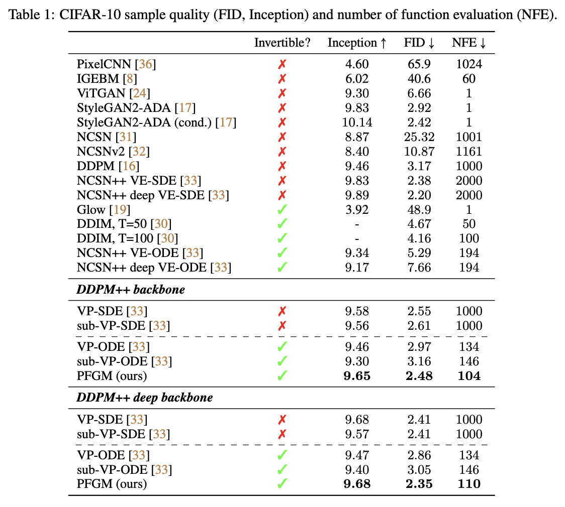
Experimental Results

PFGM is a completely new framework. It no longer relies on the Gaussian assumption as previous models did and results in a model with truly new connotations. However, we should not seek "newness for the sake of newness"; if a new framework does not produce more convincing results, then the novelty is meaningless.

The experimental results in the original paper certainly affirm the value of PFGM, showing better evaluation metrics, faster generation speeds, and better robustness to hyperparameters (including model architecture). I will not display them all here; readers can refer to the original paper. I noticed the paper was accepted to NeurIPS 2022, and it is indeed a well-deserved top-tier conference paper!

Official GitHub: https://github.com/Newbeeer/Poisson_flow

Summary

This article introduced an ODE-based diffusion model inspired by the "Law of Universal Gravitation." It breaks away from the dependence on Gaussian assumptions found in many previous diffusion models and provides a brand-new framework for constructing ODE-based diffusion models based on field theory. The entire model is highly enlightening and well worth a careful read.

Original Address: https://kexue.fm/archives/9305