Generative Diffusion Models Part 2: DDPM = Autoregressive VAE

Multi-step Breakthrough

In a traditional VAE, the encoding process and the generation process are both completed in a single step: \text{Encoding: } x \to z, \quad \text{Generation: } z \to x This approach involves only three distributions: the encoding distribution p(z|x), the generation distribution q(x|z), and the prior distribution q(z). Its advantage is that the form is relatively simple, and the mapping relationship between x and z is relatively deterministic, allowing for both the encoding and generation models to be obtained simultaneously for needs such as latent variable editing. However, its disadvantage is also obvious: because our ability to model probability distributions is limited, these three distributions can usually only be modeled as normal distributions. This limits the model’s expressive power, typically resulting in blurry generation results.

To break through this limitation, DDPM decomposes the encoding and generation processes into T steps: \begin{aligned} &\text{Encoding: } \boldsymbol{x} = \boldsymbol{x}_0 \to \boldsymbol{x}_1 \to \boldsymbol{x}_2 \to \cdots \to \boldsymbol{x}_{T-1} \to \boldsymbol{x}_T = \boldsymbol{z} \\ &\text{Generation: } \boldsymbol{z} = \boldsymbol{x}_T \to \boldsymbol{x}_{T-1} \to \boldsymbol{x}_{T-2} \to \cdots \to \boldsymbol{x}_1 \to \boldsymbol{x}_0 = \boldsymbol{x} \end{aligned} \label{eq:factor} In this way, each p(\boldsymbol{x}_t|\boldsymbol{x}_{t-1}) and q(\boldsymbol{x}_{t-1}|\boldsymbol{x}_t) is only responsible for modeling a tiny change, and they are still modeled as normal distributions. One might ask: if they are still normal distributions, why is decomposing into multiple steps better than a single step? This is because a tiny change can be sufficiently approximated by a normal distribution, similar to how a curve can be approximated by a straight line within a small range. Multi-step decomposition is somewhat like using piecewise linear functions to fit a complex curve; therefore, it can theoretically break through the fitting capacity limits of traditional single-step VAEs.

Joint Divergence

So, the plan now is to enhance the capability of the traditional VAE through the recursive decomposition in Eq. [eq:factor]. Each step of the encoding process is modeled as p(\boldsymbol{x}_t|\boldsymbol{x}_{t-1}), and each step of the generation process is modeled as q(\boldsymbol{x}_{t-1}|\boldsymbol{x}_t). The corresponding joint distributions are: \begin{aligned} &p(\boldsymbol{x}_0, \boldsymbol{x}_1, \boldsymbol{x}_2, \cdots, \boldsymbol{x}_T) = p(\boldsymbol{x}_T|\boldsymbol{x}_{T-1})\cdots p(\boldsymbol{x}_2|\boldsymbol{x}_1) p(\boldsymbol{x}_1|\boldsymbol{x}_0) \tilde{p}(\boldsymbol{x}_0) \\ &q(\boldsymbol{x}_0, \boldsymbol{x}_1, \boldsymbol{x}_2, \cdots, \boldsymbol{x}_T) = q(\boldsymbol{x}_0|\boldsymbol{x}_1)\cdots q(\boldsymbol{x}_{T-2}|\boldsymbol{x}_{T-1}) q(\boldsymbol{x}_{T-1}|\boldsymbol{x}_T) q(\boldsymbol{x}_T) \end{aligned} Don’t forget that \boldsymbol{x}_0 represents the real sample, so \tilde{p}(\boldsymbol{x}_0) is the data distribution; \boldsymbol{x}_T represents the final encoding, so q(\boldsymbol{x}_T) is the prior distribution; the remaining p(\boldsymbol{x}_t|\boldsymbol{x}_{t-1}) and q(\boldsymbol{x}_{t-1}|\boldsymbol{x}_t) represent a small step of encoding and generation, respectively. (Note: After consideration, I will continue to use the notation convention used throughout this website for introducing VAEs, i.e., "encoding distribution uses p, generation distribution uses q". Therefore, the meanings of p and q here are exactly the opposite of those in the DDPM paper. Readers should be aware of this.)

In "Variational Autoencoder (2): From a Bayesian Perspective", I proposed that the most concise theoretical way to understand VAE is to view it as minimizing the KL divergence of the joint distributions. This is also true for DDPM. We have already written the two joint distributions, so the goal of DDPM is to minimize: KL(p\Vert q) = \int p(\boldsymbol{x}_T|\boldsymbol{x}_{T-1})\cdots p(\boldsymbol{x}_1|\boldsymbol{x}_0) \tilde{p}(\boldsymbol{x}_0) \log \frac{p(\boldsymbol{x}_T|\boldsymbol{x}_{T-1})\cdots p(\boldsymbol{x}_1|\boldsymbol{x}_0) \tilde{p}(\boldsymbol{x}_0)}{q(\boldsymbol{x}_0|\boldsymbol{x}_1)\cdots q(\boldsymbol{x}_{T-1}|\boldsymbol{x}_T) q(\boldsymbol{x}_T)} d\boldsymbol{x}_0 d\boldsymbol{x}_1\cdots d\boldsymbol{x}_T \label{eq:kl} This is the optimization objective of DDPM. Up to this point, the results are the same as those in the original DDPM paper (with slightly different notation) and consistent with the more original paper "Deep Unsupervised Learning using Nonequilibrium Thermodynamics". Next, we need to define the specific forms of p(\boldsymbol{x}_t|\boldsymbol{x}_{t-1}) and q(\boldsymbol{x}_{t-1}|\boldsymbol{x}_t) and then simplify the DDPM optimization objective [eq:kl].

Divide and Conquer

First, we must know that DDPM only intends to be a generative model, so it models each step of encoding as an extremely simple normal distribution: p(\boldsymbol{x}_t|\boldsymbol{x}_{t-1})=\mathcal{N}(\boldsymbol{x}_t;\alpha_t \boldsymbol{x}_{t-1}, \beta_t^2 \boldsymbol{I}). Its main characteristic is that the mean vector is obtained simply by multiplying the input \boldsymbol{x}_{t-1} by a scalar \alpha_t. In contrast, the mean and variance of a traditional VAE are learned using neural networks. Thus, DDPM gives up the model’s encoding capability to ultimately obtain a pure generative model. As for q(\boldsymbol{x}_{t-1}|\boldsymbol{x}_t), it is modeled as a normal distribution with a learnable mean vector \mathcal{N}(\boldsymbol{x}_{t-1};\boldsymbol{\mu}(\boldsymbol{x}_t), \sigma_t^2 \boldsymbol{I}). Here, \alpha_t, \beta_t, \sigma_t are not trainable parameters but pre-set values (we will discuss how to set them later). Therefore, the only trainable parameters in the entire model are within \boldsymbol{\mu}(\boldsymbol{x}_t). (Note: The definitions of \alpha_t, \beta_t in this article are different from the original paper.)

Since the distribution p currently contains no trainable parameters, the integral in objective [eq:kl] regarding p only contributes a negligible constant. Thus, objective [eq:kl] is equivalent to: \begin{aligned} &\,-\int p(\boldsymbol{x}_T|\boldsymbol{x}_{T-1})\cdots p(\boldsymbol{x}_1|\boldsymbol{x}_0) \tilde{p}(\boldsymbol{x}_0) \log q(\boldsymbol{x}_0|\boldsymbol{x}_1)\cdots q(\boldsymbol{x}_{T-1}|\boldsymbol{x}_T) q(\boldsymbol{x}_T) d\boldsymbol{x}_0 d\boldsymbol{x}_1\cdots d\boldsymbol{x}_T \\ =&\,-\int p(\boldsymbol{x}_T|\boldsymbol{x}_{T-1})\cdots p(\boldsymbol{x}_1|\boldsymbol{x}_0) \tilde{p}(\boldsymbol{x}_0) \left[\log q(\boldsymbol{x}_T) + \sum_{t=1}^T\log q(\boldsymbol{x}_{t-1}|\boldsymbol{x}_t)\right] d\boldsymbol{x}_0 d\boldsymbol{x}_1\cdots d\boldsymbol{x}_T \end{aligned} Since the prior distribution q(\boldsymbol{x}_T) is generally taken as a standard normal distribution and also has no parameters, this term also contributes only a constant. Therefore, what needs to be calculated is each term: \begin{aligned} &\,-\int p(\boldsymbol{x}_T|\boldsymbol{x}_{T-1})\cdots p(\boldsymbol{x}_1|\boldsymbol{x}_0) \tilde{p}(\boldsymbol{x}_0) \log q(\boldsymbol{x}_{t-1}|\boldsymbol{x}_t) d\boldsymbol{x}_0 d\boldsymbol{x}_1\cdots d\boldsymbol{x}_T\\ =&\,-\int p(\boldsymbol{x}_t|\boldsymbol{x}_{t-1})\cdots p(\boldsymbol{x}_1|\boldsymbol{x}_0) \tilde{p}(\boldsymbol{x}_0) \log q(\boldsymbol{x}_{t-1}|\boldsymbol{x}_t) d\boldsymbol{x}_0 d\boldsymbol{x}_1\cdots d\boldsymbol{x}_t\\ =&\,-\int p(\boldsymbol{x}_t|\boldsymbol{x}_{t-1})p(\boldsymbol{x}_{t-1}|\boldsymbol{x}_0) \tilde{p}(\boldsymbol{x}_0) \log q(\boldsymbol{x}_{t-1}|\boldsymbol{x}_t) d\boldsymbol{x}_0 d\boldsymbol{x}_{t-1}d\boldsymbol{x}_t \end{aligned} The first equality holds because q(\boldsymbol{x}_{t-1}|\boldsymbol{x}_t) depends at most on \boldsymbol{x}_t, so the distributions from t+1 to T can be integrated to 1. The second equality holds because q(\boldsymbol{x}_{t-1}|\boldsymbol{x}_t) does not depend on \boldsymbol{x}_1, \cdots, \boldsymbol{x}_{t-2}, so we can pre-calculate the integral over them, resulting in p(\boldsymbol{x}_{t-1}|\boldsymbol{x}_0)=\mathcal{N}(\boldsymbol{x}_{t-1};\bar{\alpha}_{t-1} \boldsymbol{x}_0, \bar{\beta}_{t-1}^2 \boldsymbol{I}). This result can be referenced in Eq. [eq:x0-xt] in the next section.

Scene Re-enactment

The subsequent process is basically the same as the "How to Build" section in the previous article:

1. Removing constants irrelevant to optimization, the contribution of the term -\log q(\boldsymbol{x}_{t-1}|\boldsymbol{x}_t) is \frac{1}{2\sigma_t^2}\left\Vert\boldsymbol{x}_{t-1} - \boldsymbol{\mu}(\boldsymbol{x}_t)\right\Vert^2;

2. p(\boldsymbol{x}_{t-1}|\boldsymbol{x}_0) implies \boldsymbol{x}_{t-1} = \bar{\alpha}_{t-1}\boldsymbol{x}_0 + \bar{\beta}_{t-1}\bar{\boldsymbol{\varepsilon}}_{t-1}, and p(\boldsymbol{x}_t|\boldsymbol{x}_{t-1}) implies \boldsymbol{x}_t = \alpha_t \boldsymbol{x}_{t-1} + \beta_t \boldsymbol{\varepsilon}_t, where \bar{\boldsymbol{\varepsilon}}_{t-1}, \boldsymbol{\varepsilon}_t \sim \mathcal{N}(\boldsymbol{0}, \boldsymbol{I});

3. From \boldsymbol{x}_{t-1} = \frac{1}{\alpha_t}\left(\boldsymbol{x}_t - \beta_t \boldsymbol{\varepsilon}_t\right), we are inspired to parameterize \boldsymbol{\mu}(\boldsymbol{x}_t) as \boldsymbol{\mu}(\boldsymbol{x}_t) = \frac{1}{\alpha_t}\left(\boldsymbol{x}_t - \beta_t \boldsymbol{\epsilon}_{\boldsymbol{\theta}}(\boldsymbol{x}_t, t)\right).

Following this series of transformations, the optimization objective is equivalent to: \frac{\beta_t^2}{\alpha_t^2\sigma_t^2}\mathbb{E}_{\bar{\boldsymbol{\varepsilon}}_{t-1},\boldsymbol{\varepsilon}_t\sim \mathcal{N}(\boldsymbol{0},\boldsymbol{I}),\boldsymbol{x}_0\sim \tilde{p}(\boldsymbol{x}_0)}\left[\left\Vert \boldsymbol{\varepsilon}_t - \boldsymbol{\epsilon}_{\boldsymbol{\theta}}(\bar{\alpha}_t\boldsymbol{x}_0 + \alpha_t\bar{\beta}_{t-1}\bar{\boldsymbol{\varepsilon}}_{t-1} + \beta_t \boldsymbol{\varepsilon}_t, t)\right\Vert^2\right] Then, following the "Reducing Variance" section to perform a change of variables, the result is: \frac{\beta_t^4}{\bar{\beta}_t^2\alpha_t^2\sigma_t^2}\mathbb{E}_{\boldsymbol{\varepsilon}\sim \mathcal{N}(\boldsymbol{0},\boldsymbol{I}),\boldsymbol{x}_0\sim \tilde{p}(\boldsymbol{x}_0)}\left[\left\Vert\boldsymbol{\varepsilon} - \frac{\bar{\beta}_t}{\beta_t}\boldsymbol{\epsilon}_{\boldsymbol{\theta}}(\bar{\alpha}_t\boldsymbol{x}_0 + \bar{\beta}_t\boldsymbol{\varepsilon}, t)\right\Vert^2\right] \label{eq:loss} This gives the training objective for DDPM (the original paper found through experiments that the actual effect is better if the coefficient in front of the above formula is removed). It was obtained by starting from the VAE optimization objective and gradually simplifying the integral results. Although it is somewhat long, every step follows a logical path; there is computational difficulty, but no conceptual difficulty.

In contrast, the original DDPM paper abruptly introduced q(\boldsymbol{x}_{t-1}|\boldsymbol{x}_t, \boldsymbol{x}_0) (original paper notation) to perform term cancellation, then converted it into the KL divergence form of normal distributions. This step in the entire process is highly technical and seems "mysterious," which was quite difficult for me to accept.

Hyperparameter Settings

In this section, we discuss the selection of \alpha_t, \beta_t, \sigma_t.

For p(\boldsymbol{x}_t|\boldsymbol{x}_{t-1}), it is customary to set \alpha_t^2 + \beta_t^2=1, which reduces the number of parameters by half and helps simplify the form. We already derived this in the previous article. Due to the additivity of normal distributions, under this constraint we have: p(\boldsymbol{x}_t|\boldsymbol{x}_0) = \int p(\boldsymbol{x}_t|\boldsymbol{x}_{t-1})\cdots p(\boldsymbol{x}_1|\boldsymbol{x}_0) d\boldsymbol{x}_1\cdots d\boldsymbol{x}_{t-1} = \mathcal{N}(\boldsymbol{x}_t;\bar{\alpha}_t \boldsymbol{x}_0, \bar{\beta}_t^2 \boldsymbol{I}) \label{eq:x0-xt} where \bar{\alpha}_t = \alpha_1\cdots\alpha_t and \bar{\beta}_t = \sqrt{1-\bar{\alpha}_t^2}. In this way, p(\boldsymbol{x}_t|\boldsymbol{x}_0) has a relatively simple form. One might ask how the constraint \alpha_t^2 + \beta_t^2=1 was thought of beforehand. We know that \mathcal{N}(\boldsymbol{x}_t;\alpha_t \boldsymbol{x}_{t-1}, \beta_t^2 \boldsymbol{I}) means \boldsymbol{x}_t = \alpha_t \boldsymbol{x}_{t-1} + \beta_t \boldsymbol{\varepsilon}_t, \boldsymbol{\varepsilon}_t\sim \mathcal{N}(\boldsymbol{0},\boldsymbol{I}). If \boldsymbol{x}_{t-1} is also \sim \mathcal{N}(\boldsymbol{0},\boldsymbol{I}), we would want \boldsymbol{x}_t to be \sim \mathcal{N}(\boldsymbol{0},\boldsymbol{I}) as well, which determines \alpha_t^2+\beta_t^2=1.

As mentioned earlier, q(\boldsymbol{x}_T) is generally taken as the standard normal distribution \mathcal{N}(\boldsymbol{x}_T;\boldsymbol{0}, \boldsymbol{I}). Since our learning goal is to minimize the KL divergence between the two joint distributions, i.e., we hope p=q, their marginal distributions should naturally be equal. Therefore, we also hope: q(\boldsymbol{x}_T) = \int p(\boldsymbol{x}_T|\boldsymbol{x}_{T-1})\cdots p(\boldsymbol{x}_1|\boldsymbol{x}_0) \tilde{p}(\boldsymbol{x}_0) d\boldsymbol{x}_0 d\boldsymbol{x}_1\cdots d\boldsymbol{x}_{T-1} = \int p(\boldsymbol{x}_T|\boldsymbol{x}_0) \tilde{p}(\boldsymbol{x}_0) d\boldsymbol{x}_0 Since the data distribution \tilde{p}(\boldsymbol{x}_0) is arbitrary, for the above equation to hold identically, p(\boldsymbol{x}_T|\boldsymbol{x}_0) must equal q(\boldsymbol{x}_T), i.e., it must degenerate into a standard normal distribution independent of \boldsymbol{x}_0. This means we need to design an appropriate \alpha_t such that \bar{\alpha}_T\approx 0. At the same time, this tells us again that DDPM has no encoding capability; the final p(\boldsymbol{x}_T|\boldsymbol{x}_0) can be said to be independent of the input \boldsymbol{x}_0. Using the "demolition-construction" analogy from the previous article, it means the original building has been completely demolished into raw materials. If these materials are used to rebuild, any building can be constructed, not necessarily the one that existed before demolition. DDPM chose \alpha_t = \sqrt{1 - \frac{0.02t}{T}}. The properties of this choice were also analyzed in the "Hyperparameter Settings" section of the previous article.

As for \sigma_t, theoretically, different data distributions \tilde{p}(\boldsymbol{x}_0) correspond to different optimal \sigma_t. However, we do not want to set \sigma_t as a trainable parameter, so we have to choose some special \tilde{p}(\boldsymbol{x}_0) to derive the corresponding optimal \sigma_t and assume that the \sigma_t derived from special cases can generalize to general data distributions. We can consider two simple examples:

1. Assume the training set has only one sample \boldsymbol{x}_*, i.e., \tilde{p}(\boldsymbol{x}_0) is the Dirac delta distribution \delta(\boldsymbol{x}_0 - \boldsymbol{x}_*). This leads to the optimal \sigma_t = \frac{\bar{\beta}_{t-1}}{\bar{\beta}_t}\beta_t;

2. Assume the data distribution \tilde{p}(\boldsymbol{x}_0) follows a standard normal distribution. In this case, the optimal \sigma_t = \beta_t.

Experimental results show that the performance of the two choices is similar, so either can be chosen for sampling. The derivation process for these two results is quite long, and we will discuss them at another time.

Reference Implementation

How can such a wonderful model lack a Keras implementation? Below is my reference implementation:

Github Address: https://github.com/bojone/Keras-DDPM

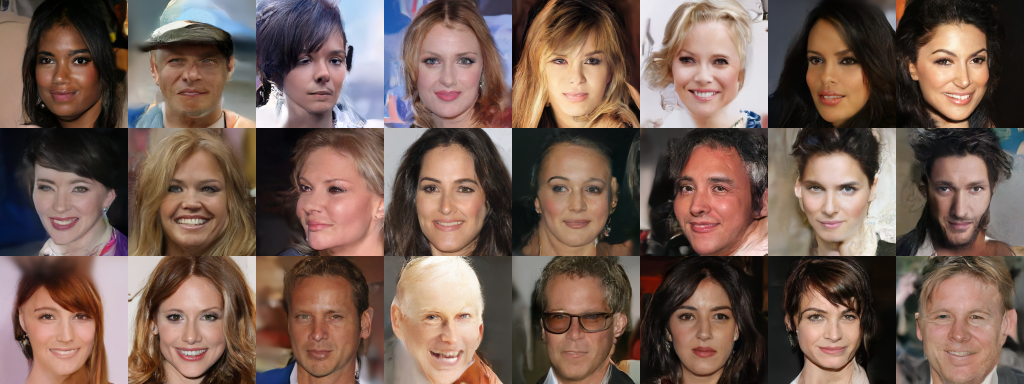
Note that my implementation does not strictly follow the original DDPM open-source code. Instead, I simplified the U-Net architecture based on my own design (e.g., changing feature concatenation to addition, removing Attention, etc.) to achieve results quickly. Testing on a single 3090 with 24G VRAM, training on the 128*128 CelebA HQ face dataset with blocks=1, batch_size=64, results began to appear within half a day. The sampling effect after 3 days of training is as follows:

During the debugging process, I summarized the following practical experiences:

1. The loss function should not use MSE; instead, the squared Euclidean distance must be used. The difference is that MSE is the squared Euclidean distance divided by (\text{width} \times \text{height} \times \text{channels}). This leads to a loss value that is too small, and gradients for some parameters might be ignored as zero, causing the training process to converge first and then diverge. This phenomenon also frequently occurs in low-precision training; refer to "Using Mixed Precision and XLA to Accelerate Training in bert4keras".

2. For normalization, Instance Norm, Layer Norm, or Group Norm can be used, but do not use Batch Norm. Batch Norm has the problem of inconsistency between training and inference, which may lead to excellent training effects but very poor prediction effects.

3. There is no need to copy the network structure from the original paper exactly. The original paper was aimed at hitting SOTA for publication; copying it would definitely be large and slow. Simply designing an autoencoder following the U-Net idea is basically enough to train a decent result, as it is essentially a pure regression problem and thus quite easy to train.

4. Regarding the input of parameter t, the original paper used Sinusoidal position encoding. I found that replacing it directly with a trainable Embedding yields similar results.

5. Following the habit of pre-training language models, I used the LAMB optimizer. it makes tuning the learning rate more convenient; basically, a learning rate of 10^{-3} is applicable to model training with any initialization method.

Comprehensive Evaluation

Combining "Generative Diffusion Models Part 1: DDPM = Demolition + Construction" and this article, readers should now have their own views on DDPM. You can basically see where the advantages, disadvantages, and corresponding improvement directions of DDPM lie.

The advantages of DDPM are obvious: it is easy to train, and the generated images are clear. This ease of training is relative to GANs. A GAN is a \min-\max process with high uncertainty and a tendency to collapse, whereas DDPM is a pure regression loss function requiring only pure minimization, making the training process very stable. At the same time, through the "demolition-construction" analogy, we can find that DDPM is not inferior to GANs in terms of popular understanding.

However, the disadvantages of DDPM are also obvious. First and foremost is the slow sampling speed, which requires executing the model T steps (T=1000 in the original paper) to complete sampling. This is T times slower than the one-step sampling of GANs. Many subsequent works have focused on improving this. Secondly, in GANs, the training from random noise to generated samples is a deterministic transformation; the random noise is a decoupled latent variable of the generation result, allowing us to perform interpolation or edit it to achieve controlled generation. But in DDPM, the generation process is completely stochastic, and there is no deterministic relationship between the two, so such editing does not exist. Although the original DDPM paper demonstrated interpolation effects, those were performed on original images by using noise to blur them and letting the model "re-imagine" new images; such interpolation is difficult to achieve in terms of semantic fusion.

In addition to making improvements targeting these disadvantages, there are other directions for DDPM. For example, the DDPMs demonstrated so far are unconditional. Naturally, one thinks of conditional DDPMs, just like the transition from VAE to C-VAE or GAN to C-GAN. This is a mainstream application of current diffusion models. For instance, Google’s Imagen includes using diffusion models for text-to-image generation and super-resolution, both of which are essentially conditional diffusion models. Furthermore, while the current DDPM is designed for continuous variables, its idea should also be applicable to discrete data. How should a DDPM for discrete data be designed?

Related Work

Speaking of related work for DDPM, most people think of traditional diffusion models, energy-based models, or denoising autoencoders. However, what I want to mention next is something previously introduced in this blog, which could even be considered a case where DDPM is a special instance: "The Powerful NVAE: Never Say VAE Generated Images are Blurry Again".

From the VAE perspective, traditional VAE-generated images are mostly blurry, and DDPM is only the second VAE (that I know of) capable of generating clear images; the first was NVAE. Looking at the form of NVAE, we can find many similarities with DDPM. For example, NVAE also introduces a large number of latent variables z=\{z_1, z_2, \dots, z_L\}, and these variables also have a recursive relationship, so the sampling process of NVAE is very similar to that of DDPM.

In terms of theoretical form, DDPM can be seen as an extremely simplified NVAE, where the recursive relationship of latent variables is modeled only as a Markovian conditional normal distribution, rather than the non-Markovian form of NVAE. The generative model is also just repeated iterations of the same model, rather than a massive model using z=\{z_1, z_2, \dots, z_L\} simultaneously like NVAE. However, while NVAE uses many z=\{z_1, z_2, \dots, z_L\}, it also incorporates a parameter-sharing mechanism, which is essentially similar to the repeated iteration of the same model.

Summary

This article derived DDPM from the perspective of the Variational Autoencoder (VAE). In this view, DDPM is a simplified version of an autoregressive VAE, very similar to the previous NVAE. At the same time, this article shared my own DDPM implementation code and practical experience, along with a comprehensive evaluation of DDPM.

Original Address: https://kexue.fm/archives/9152