A Brief Analysis of the Hubness Phenomenon in the ``Curse of Dimensionality''

The Collapsing Ball

The “Curse of Dimensionality” is a very broad concept. Any conclusion in high-dimensional space that differs significantly from its two-dimensional or three-dimensional counterparts can be called a “Curse of Dimensionality.” For example, as introduced in “Distribution of the Angle Between Two Random Vectors in n-Dimensional Space,” any two vectors in a high-dimensional space are almost always orthogonal. Many of these phenomena share the same root cause: “the ratio of the volume of an n-dimensional unit ball to its circumscribed cube collapses to 0 as n increases.” This is also true for the “Hubness phenomenon” discussed in this article.

In “The Masterpiece: Calculating the Volume of an n-Dimensional Ball,” we derived the formula for the volume of an n-dimensional ball. From this, we know that the volume of an n-dimensional unit ball is: V_n = \frac{\pi^{n/2}}{\Gamma\left(\frac{n}{2}+1\right)} The side length of the corresponding circumscribed cube is 2, so its volume is 2^n. Thus, the volume ratio is V_n / 2^n. The plot of this ratio is shown below:

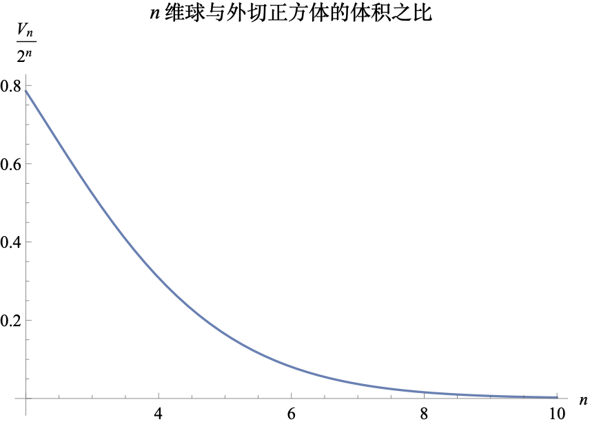
As seen, as the dimension increases, this ratio quickly approaches 0. A vivid description of this conclusion is that “as the dimension increases, the ball becomes increasingly insignificant.” This tells us that if we attempt to achieve uniform sampling within a ball using a “uniform distribution + rejection sampling” method, the efficiency in high-dimensional space will be extremely low (the rejection rate approaches 100%). Another way to understand this is that “most points inside a high-dimensional ball are concentrated near the surface of the ball,” and the proportion of the region from the center to the vicinity of the surface becomes smaller and smaller.

The Hubness Phenomenon

Now we turn to the Hubness phenomenon. It states that if a set of points is randomly selected in a high-dimensional space, “there are always some points that frequently appear in the k-nearest neighbors of other points.”

How should we understand this? Suppose we have N points x_1, x_2, \dots, x_N. For each x_i, we can find the k points closest to it; these k points are called the “k-neighbors of x_i.” With the concept of k-neighbors, we can count how many times each point appears in the k-neighbors of other points. This count is called the “Hub value.” In other words, the larger the Hub value, the more likely the point is to appear in the k-neighbors of others.

Thus, the Hubness phenomenon says: there are always a few points whose Hub values are significantly large. If the Hub value represents “wealth,” a vivid metaphor would be “80% of the wealth is concentrated in the hands of 20% of the people,” and as the dimension increases, this “wealth gap” grows larger. If the Hub value represents “connections,” it can be likened to “there are always a few individuals in a community who possess very extensive social resources.”

How does the Hubness phenomenon arise? It is actually related to the collapse of the n-dimensional ball mentioned in the previous section. We know that the point that minimizes the sum of squared distances to all points is exactly the mean point: \frac{1}{N} \sum_{i=1}^N x_i = c^* = \mathop{\text{argmin}}_c \sum_{i=1}^N \Vert x_i - c\Vert^2 This implies that points near the mean vector have a smaller average distance to all points and thus have a greater chance of becoming k-neighbors for more points. The collapse of the n-dimensional ball tells us that the “points near the mean vector”—specifically, a spherical neighborhood centered at the mean vector—occupy an extremely small proportion of the space. Consequently, the phenomenon of “very few points appearing in the k-neighbors of many points” occurs. Of course, the mean vector here is an intuitive explanation; in general data points, points closer to the density center will have larger Hub values.

Improving Sampling

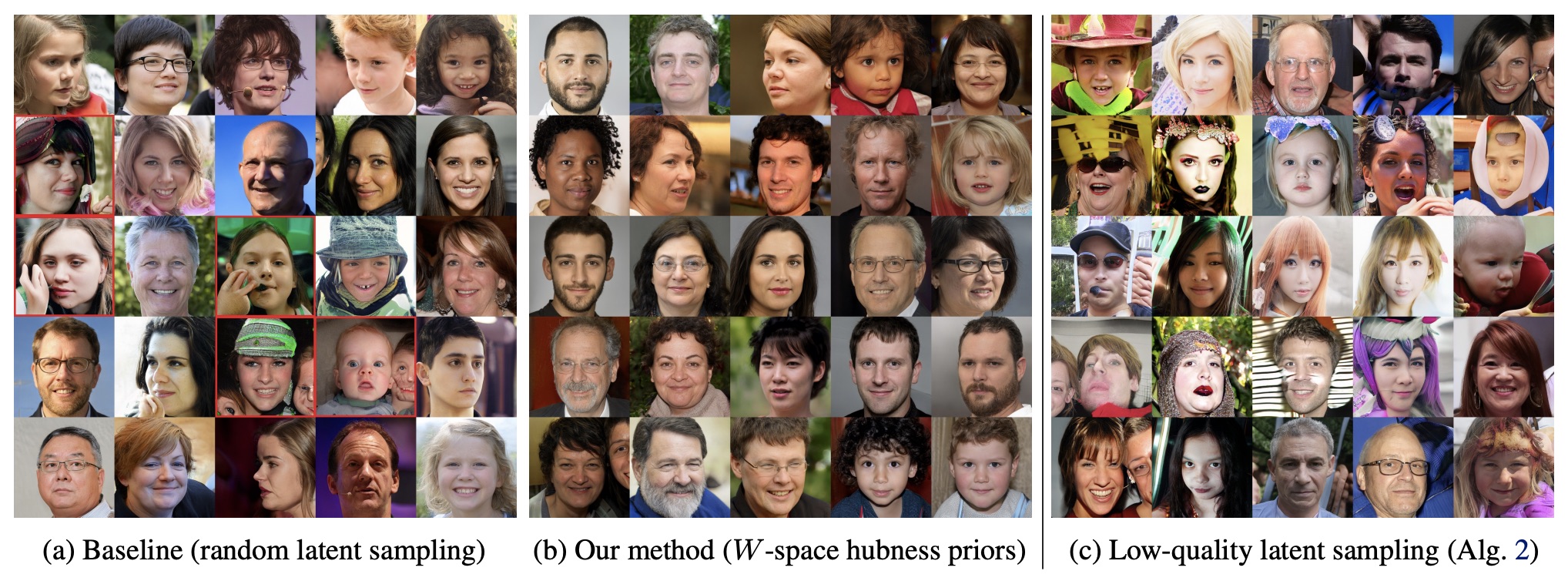
So, what is the relationship between the scheme for improving GAN generation quality mentioned at the beginning and the Hubness phenomenon? The paper “Exploring and Exploiting Hubness Priors for High-Quality GAN Latent Sampling” proposes a prior hypothesis: the larger the Hub value, the better the generation quality of the corresponding point.

Specifically, the general GAN sampling generation process is z \sim \mathcal{N}(0,1), x=G(z). We can first sample N points z_1, z_2, \dots, z_N from \mathcal{N}(0,1) and then calculate the Hub value for each sample point. The original paper found that the Hub value is positively correlated with generation quality, so only sample points with a Hub value greater than or equal to a threshold t are kept for generation. This is a “pre-filtering” strategy. Reference code is as follows:

def get_z_samples(size, t=50):
    """Filter sampling results via Hub values
    """
    Z = np.empty((0, z_dim))
    while len(Z) < size:
        z = np.random.randn(10000, z_dim)
        s = np.zeros(10000)
        for i in range(10):
            zi = z[i * 1000:(i + 1) * 1000]
            d = (z**2).sum(1)[:, None] + (zi**2).sum(1)[None] - 2 * z.dot(zi.T)
            for j in d.argsort(0)[1:1 + 5].T:
                s[j] += 1
        z = z[s > t]
        Z = np.concatenate([Z, z], 0)[:size]
        print('%s / %s' % (len(Z), size))
    return Z

Why filter by Hub value? From the previous discussion, we know that a larger Hub value means the point is closer to the sample center—more accurately, the density center. This implies there are many neighboring points around it, making it unlikely to be an under-trained outlier. Therefore, the sampling quality is relatively higher. Multiple experimental results in the paper confirm this conclusion.

Summary

This article briefly introduced the Hubness phenomenon within the “Curse of Dimensionality” and its application in improving the generation quality of GANs.

Reprinted from: https://kexue.fm/archives/9147
For more details on reprinting, please refer to: Scientific Space FAQ