The Success of WGAN May Have Little to Do with the Wasserstein Distance

Basics and Review

This article is a discussion of the WGAN training process and is not intended as an introductory piece. For those new to GANs, please refer to The Art of Mutual Confrontation: From Zero to WGAN-GP. For the connection between f-divergence and GANs, you can refer to Introduction to f-GAN: The Production Workshop of GAN Models and Designing GANs: Another GAN Production Workshop. For the theoretical derivation of WGAN, see From Wasserstein Distance and Duality Theory to WGAN. For an analysis of the GAN training process, you can also refer to Optimization Algorithms from a Dynamical Perspective (IV): The Third Stage of GAN.

Generally speaking, a GAN corresponds to a min-max process: \min_G \max_D \mathcal{L}(D, G) Of course, the loss functions for the discriminator and the generator might differ in practice, but the above form is sufficiently representative. The original GAN is generally called the vanilla GAN, and its form is: \min_G \max_D \mathbb{E}_{x\sim p(x)}\left[\log D(x)\right] + \mathbb{E}_{z\sim q(z)}\left[\log (1 - D(G(z)))\right]\label{eq:v-gan} As proven in Towards Principled Methods for Training Generative Adversarial Networks, The Amazing Wasserstein GAN, or related articles on this blog, the vanilla GAN essentially minimizes the JS divergence between two distributions. JS divergence is a type of f-divergence, and all f-divergences share a common problem: when two distributions have almost no overlap, the divergence becomes a constant. This implies that the gradient is zero. Since we use gradient descent for optimization, this means we cannot complete the optimization effectively. To address this, WGAN was born, utilizing the Wasserstein distance to design a new GAN: \min_G \max_{\Vert D\Vert_{L}\leq 1} \mathbb{E}_{x\sim p(x)}\left[D(x)\right] - \mathbb{E}_{z\sim q(z)}\left[D(G(z))\right]\label{eq:w-gan} The obvious difference from previous GANs is that WGAN explicitly adds a Lipschitz constraint \Vert D\Vert_{L}\leq 1 to the discriminator D. Since the Wasserstein distance is well-defined for almost any two distributions (even those without overlap), WGAN theoretically solves the problems of vanishing gradients and training instability found in traditional f-divergence-based GANs.

There are two main schemes for adding the Lipschitz constraint to the discriminator: first, Spectral Normalization (SN), which can be referenced in Lipschitz Constraints in Deep Learning: Generalization and Generative Models. Many GANs today (not limited to WGAN) incorporate Spectral Normalization into the discriminator or even the generator to stabilize training. Second, Gradient Penalty (GP), which includes penalties centered at 1 (WGAN-GP) and penalties centered at 0 (WGAN-div). Refer to WGAN-div: An Obscure WGAN Successor. Current results suggest that zero-centered penalties possess better theoretical properties and performance.

Performance \neq Approximation

The phenomenon that "WGAN does not approximate the Wasserstein distance well" is not being noticed for the first time. For instance, a 2019 paper titled How Well Do WGANs Estimate the Wasserstein Metric? discussed this systematically. The paper introduced here uses rigorously designed experiments to determine the relationship between WGAN performance and the degree of Wasserstein distance approximation.

First, the paper compares the performance of Gradient Penalty (GP) with a method called c\text{-transform} in implementing WGAN. The c\text{-transform} was also proposed in How Well Do WGANs Estimate the Wasserstein Metric? and approximates the Wasserstein distance much better than Gradient Penalty. The following two figures illustrate this:

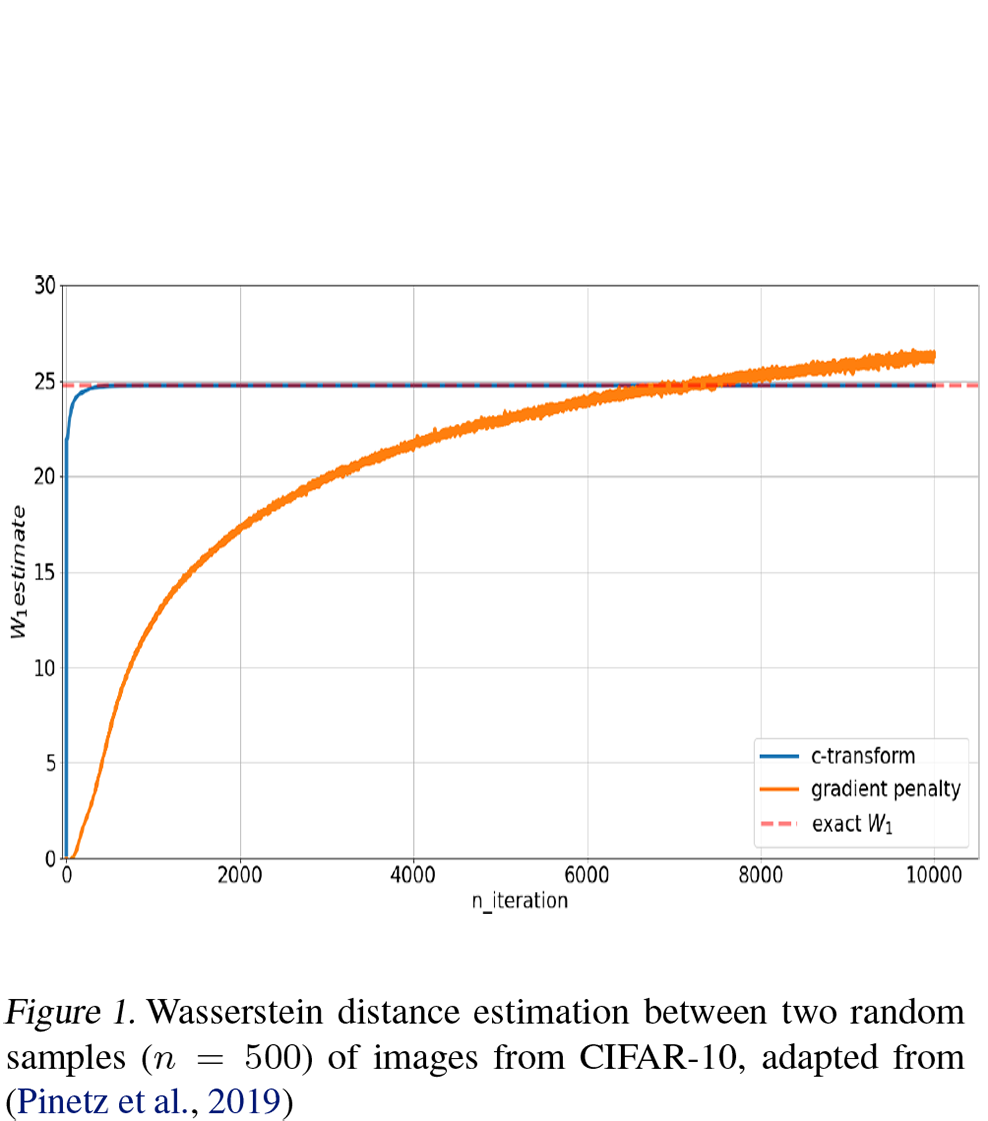
However, the generation quality of c\text{-transform} is not as good as that of Gradient Penalty:

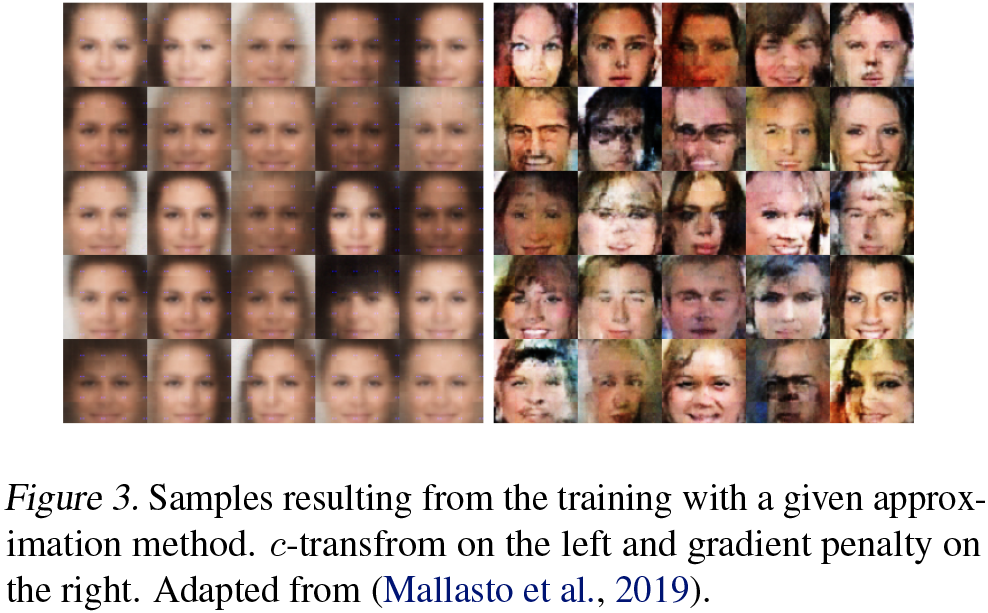
Admittedly, the choice of this image in the original paper is somewhat amusing; in fact, the results of WGAN-GP can be much better than what is shown on the right. Thus, we can temporarily conclude:

1. High-performing WGANs do not approximate the Wasserstein distance well during the training process;
2. Better approximation of the Wasserstein distance does not actually help in improving generation performance.

Theory \neq Experiment

Now let us consider where the problem lies. We know that whether it is the original GAN [eq:v-gan], WGAN [eq:w-gan], or other GAN variants, they all share two common characteristics during experimentation:

1. \min and \max are trained alternately;
2. Only a random batch is selected for training each time.

What are the issues with these two points?

First, almost all GANs are written as \min\limits_G \max\limits_D. This is because, theoretically, one needs to complete \max\limits_D precisely before proceeding to \min\limits_G to optimize the probability measure corresponding to the GAN. If optimization is merely alternating, it is theoretically impossible to approximate the probability measure accurately. Even though WGAN uses the Wasserstein distance and is less prone to vanishing gradients—allowing for several extra training steps for D (or a higher learning rate for D)—it still cannot precisely approximate the Wasserstein distance. This is one source of the discrepancy.

Second, training on a random batch rather than the full set of training samples leads to a specific result: "the Wasserstein distance between two randomly selected batches from the training set is greater than the Wasserstein distance between a training batch and its average sample," as shown below:

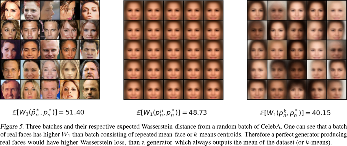
This indicates that under batch-based training, if you want to obtain more realistic samples, you are inevitably not optimizing the Wasserstein distance. If you were optimizing the Wasserstein distance very precisely, you would not obtain realistic samples because the Wasserstein distance for blurry average samples is actually smaller.

Math \neq Vision

Mathematically, the properties of the Wasserstein distance are indeed very elegant. In a sense, it is the optimal solution for measuring the gap between any two distributions. However, math is math, and the most "critical" aspect of the Wasserstein distance is its dependence on a specific metric: \mathcal{W}[p,q]=\inf_{\gamma\in \Pi[p,q]} \iint \gamma(x,y) d(x,y) dxdy That is, we need to provide a function d(x,y) that measures the distance between two samples. However, for many scenarios, such as images, designing this distance function is the hardest of all tasks. WGAN directly uses the Euclidean distance d(x,y)=\Vert x - y\Vert_2, which, although mathematically reasonable, is visually problematic. Two images that we perceive as similar might not have a small Euclidean distance. Therefore, accurately approximating the Wasserstein distance can actually lead to poorer visual results. The original paper also conducted experiments showing that when the c-transform is used to better approximate the Wasserstein distance, the generated results are similar to K-Means clustering centers, which also use Euclidean distance as a metric:

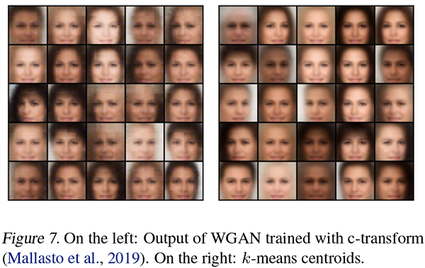
So, the reason for WGAN’s success is now quite mysterious: WGAN is derived from the Wasserstein distance, but in implementation, there is a gap from the Wasserstein distance, and this gap might be the key to WGAN’s success. The original paper argues that the most critical aspect of WGAN is the introduction of the Lipschitz constraint. Adding a Lipschitz constraint (Spectral Normalization or Gradient Penalty) to almost any GAN variant tends to improve performance and stability. Therefore, the Lipschitz constraint is the key to improvement, rather than the Wasserstein distance as imagined.

However, this is more of a conclusion than a theoretical analysis. It seems that a deep understanding of GANs still has a long way to go.

Simple Summary

This article mainly shared a recent paper pointing out that whether the Wasserstein distance is approximated or not has no necessary connection with the performance of WGAN. How to better understand the theory and practice of GANs remains a difficult task.

Original address: https://kexue.fm/archives/8244
For more details on reprinting, please refer to: Scientific Space FAQ