In the previous article, we provided a detailed derivation and understanding of the original Sinusoidal position encoding. The general feeling was that Sinusoidal encoding is an "absolute position encoding that wants to be a relative position encoding." Generally speaking, absolute position encoding has the advantages of simple implementation and fast calculation, while relative position encoding directly reflects relative position signals, which aligns with our intuitive understanding and often yields better actual performance. From this, it is evident that if relative position encoding can be implemented via an absolute position encoding method, we would "gather the strengths of all parties" and "have our cake and eat it too." Sinusoidal position encoding vaguely achieved this, but not well enough.
This article introduces our self-developed Rotary Transformer (RoFormer) model. Its primary modification is the application of the "Rotary Position Embedding (RoPE)" conceived by the author. This is a design that, when paired with the Attention mechanism, achieves "relative position encoding through absolute position encoding." Because of this design, it is currently the only relative position encoding that can be used for Linear Attention.
Basic Idea
In a previous article, "Transformer Position Encodings that Rack Researchers’ Brains", we briefly introduced RoPE, calling it "fused" at the time. This article introduces its origin and properties in more detail. In RoPE, our starting point is to "achieve relative position encoding through absolute position encoding." This approach has both theoretical elegance and practical utility; for instance, its extensibility to Linear Attention is primarily due to this point.
To achieve this goal, we assume that absolute position information is added to \boldsymbol{q} and \boldsymbol{k} through the following operations: \tilde{\boldsymbol{q}}_m = \boldsymbol{f}(\boldsymbol{q}, m), \quad \tilde{\boldsymbol{k}}_n = \boldsymbol{f}(\boldsymbol{k}, n) That is, we design operations \boldsymbol{f}(\cdot, m) and \boldsymbol{f}(\cdot, n) for \boldsymbol{q} and \boldsymbol{k} respectively, such that after the operation, \tilde{\boldsymbol{q}}_m and \tilde{\boldsymbol{k}}_n carry absolute position information for positions m and n. Since the core operation of Attention is the inner product, we hope the result of the inner product carries relative position information. Therefore, we assume the existence of an identity relationship: \langle\boldsymbol{f}(\boldsymbol{q}, m), \boldsymbol{f}(\boldsymbol{k}, n)\rangle = g(\boldsymbol{q},\boldsymbol{k},m-n) Thus, we need to find a (preferably simple) solution to this identity. The solution process also requires some initial conditions; clearly, we can reasonably set \boldsymbol{f}(\boldsymbol{q}, 0)=\boldsymbol{q} and \boldsymbol{f}(\boldsymbol{k}, 0)=\boldsymbol{k}.
Derivation Process
Following the same logic as the previous article, we first consider the two-dimensional case and solve it using complex numbers. In complex numbers, we have \langle\boldsymbol{q},\boldsymbol{k}\rangle=\text{Re}[\boldsymbol{q}\boldsymbol{k}^*], where \text{Re}[] represents the real part of a complex number. So we have: \text{Re}[\boldsymbol{f}(\boldsymbol{q}, m)\boldsymbol{f}^*(\boldsymbol{k}, n)] = g(\boldsymbol{q},\boldsymbol{k},m-n) For simplicity, we assume there exists a complex number \boldsymbol{g}(\boldsymbol{q},\boldsymbol{k},m-n) such that \boldsymbol{f}(\boldsymbol{q}, m)\boldsymbol{f}^*(\boldsymbol{k}, n) = \boldsymbol{g}(\boldsymbol{q},\boldsymbol{k},m-n). Using the exponential form of complex numbers, let: \begin{aligned} \boldsymbol{f}(\boldsymbol{q}, m) =&\, R_f (\boldsymbol{q}, m)e^{\text{i}\Theta_f(\boldsymbol{q}, m)} \\ \boldsymbol{f}(\boldsymbol{k}, n) =&\, R_f (\boldsymbol{k}, n)e^{\text{i}\Theta_f(\boldsymbol{k}, n)} \\ \boldsymbol{g}(\boldsymbol{q}, \boldsymbol{k}, m-n) =&\, R_g (\boldsymbol{q}, \boldsymbol{k}, m-n)e^{\text{i}\Theta_g(\boldsymbol{q}, \boldsymbol{k}, m-n)} \\ \end{aligned} Substituting these into the equation yields the system: \begin{aligned} R_f (\boldsymbol{q}, m) R_f (\boldsymbol{k}, n) =&\, R_g (\boldsymbol{q}, \boldsymbol{k}, m-n) \\ \Theta_f (\boldsymbol{q}, m) - \Theta_f (\boldsymbol{k}, n) =&\, \Theta_g (\boldsymbol{q}, \boldsymbol{k}, m-n) \end{aligned} For the first equation, substituting m=n gives: R_f (\boldsymbol{q}, m) R_f (\boldsymbol{k}, m) = R_g (\boldsymbol{q}, \boldsymbol{k}, 0) = R_f (\boldsymbol{q}, 0) R_f (\boldsymbol{k}, 0) = \Vert \boldsymbol{q}\Vert \Vert \boldsymbol{k}\Vert The last equality stems from the initial conditions \boldsymbol{f}(\boldsymbol{q}, 0)=\boldsymbol{q} and \boldsymbol{f}(\boldsymbol{k}, 0)=\boldsymbol{k}. Thus, we can simply set R_f (\boldsymbol{q}, m)=\Vert \boldsymbol{q}\Vert and R_f (\boldsymbol{k}, m)=\Vert \boldsymbol{k}\Vert, meaning they do not depend on m. As for the second equation, substituting m=n gives: \Theta_f (\boldsymbol{q}, m) - \Theta_f (\boldsymbol{k}, m) = \Theta_g (\boldsymbol{q}, \boldsymbol{k}, 0) = \Theta_f (\boldsymbol{q}, 0) - \Theta_f (\boldsymbol{k}, 0) = \Theta (\boldsymbol{q}) - \Theta (\boldsymbol{k}) Here \Theta (\boldsymbol{q}) and \Theta (\boldsymbol{k}) are the arguments (phases) of \boldsymbol{q} and \boldsymbol{k} themselves. From the above, we get \Theta_f (\boldsymbol{q}, m) - \Theta (\boldsymbol{q}) = \Theta_f (\boldsymbol{k}, m) - \Theta (\boldsymbol{k}), so \Theta_f (\boldsymbol{q}, m) - \Theta (\boldsymbol{q}) should be a function related only to m and independent of \boldsymbol{q}, denoted as \varphi(m), i.e., \Theta_f (\boldsymbol{q}, m) = \Theta (\boldsymbol{q}) + \varphi(m). Substituting n=m-1 and rearranging gives: \varphi(m) - \varphi(m-1) = \Theta_g (\boldsymbol{q}, \boldsymbol{k}, 1) + \Theta (\boldsymbol{k}) - \Theta (\boldsymbol{q}) This implies that \{\varphi(m)\} is an arithmetic progression. Setting the right side as \theta, we solve to find \varphi(m)=m\theta.
Encoding Form
In summary, we obtain RoPE for the 2D case expressed in complex numbers: \boldsymbol{f}(\boldsymbol{q}, m) = R_f (\boldsymbol{q}, m)e^{\text{i}\Theta_f(\boldsymbol{q}, m)} = \Vert q\Vert e^{\text{i}(\Theta(\boldsymbol{q}) + m\theta)} = \boldsymbol{q} e^{\text{i}m\theta} According to the geometric meaning of complex multiplication, this transformation corresponds to the rotation of a vector. Thus, we call it "Rotary Position Embedding." It can also be written in matrix form: \boldsymbol{f}(\boldsymbol{q}, m) =\begin{pmatrix}\cos m\theta & -\sin m\theta\\ \sin m\theta & \cos m\theta\end{pmatrix} \begin{pmatrix}q_0 \\ q_1\end{pmatrix} Since the inner product satisfies linear additivity, any even-dimensional RoPE can be represented as a concatenation of 2D cases: \scriptsize{\underbrace{\begin{pmatrix} \cos m\theta_0 & -\sin m\theta_0 & 0 & 0 & \cdots & 0 & 0 \\ \sin m\theta_0 & \cos m\theta_0 & 0 & 0 & \cdots & 0 & 0 \\ 0 & 0 & \cos m\theta_1 & -\sin m\theta_1 & \cdots & 0 & 0 \\ 0 & 0 & \sin m\theta_1 & \cos m\theta_1 & \cdots & 0 & 0 \\ \vdots & \vdots & \vdots & \vdots & \ddots & \vdots & \vdots \\ 0 & 0 & 0 & 0 & \cdots & \cos m\theta_{d/2-1} & -\sin m\theta_{d/2-1} \\ 0 & 0 & 0 & 0 & \cdots & \sin m\theta_{d/2-1} & \cos m\theta_{d/2-1} \\ \end{pmatrix}}_{\boldsymbol{\mathcal{R}}_m} \begin{pmatrix}q_0 \\ q_1 \\ q_2 \\ q_3 \\ \vdots \\ q_{d-2} \\ q_{d-1}\end{pmatrix}} That is, by multiplying the vector \boldsymbol{q} at position m by matrix \boldsymbol{\mathcal{R}}_m and the vector \boldsymbol{k} at position n by matrix \boldsymbol{\mathcal{R}}_n, the Attention mechanism using the transformed \boldsymbol{Q} and \boldsymbol{K} sequences will automatically include relative position information, because the following identity holds: (\boldsymbol{\mathcal{R}}_m \boldsymbol{q})^{\top}(\boldsymbol{\mathcal{R}}_n \boldsymbol{k}) = \boldsymbol{q}^{\top} \boldsymbol{\mathcal{R}}_m^{\top}\boldsymbol{\mathcal{R}}_n \boldsymbol{k} = \boldsymbol{q}^{\top} \boldsymbol{\mathcal{R}}_{n-m} \boldsymbol{k} It is worth noting that \boldsymbol{\mathcal{R}}_m is an orthogonal matrix; it does not change the norm of the vector, so it generally does not affect the stability of the original model.
Due to the sparsity of \boldsymbol{\mathcal{R}}_m, using direct matrix multiplication would be computationally wasteful. It is recommended to implement RoPE as follows: \begin{pmatrix}q_0 \\ q_1 \\ q_2 \\ q_3 \\ \vdots \\ q_{d-2} \\ q_{d-1} \end{pmatrix}\otimes\begin{pmatrix}\cos m\theta_0 \\ \cos m\theta_0 \\ \cos m\theta_1 \\ \cos m\theta_1 \\ \vdots \\ \cos m\theta_{d/2-1} \\ \cos m\theta_{d/2-1} \end{pmatrix} + \begin{pmatrix}-q_1 \\ q_0 \\ -q_3 \\ q_2 \\ \vdots \\ -q_{d-1} \\ q_{d-2} \end{pmatrix}\otimes\begin{pmatrix}\sin m\theta_0 \\ \sin m\theta_0 \\ \sin m\theta_1 \\ \sin m\theta_1 \\ \vdots \\ \sin m\theta_{d/2-1} \\ \sin m\theta_{d/2-1} \end{pmatrix} where \otimes denotes element-wise multiplication (the * operation in frameworks like Numpy or TensorFlow). From this implementation, RoPE can be seen as a variant of multiplicative position encoding.
Long-term Decay
As can be seen, RoPE is somewhat similar in form to Sinusoidal position encoding, except that Sinusoidal is additive while RoPE can be viewed as multiplicative. For the choice of \theta_i, we follow the Sinusoidal scheme, i.e., \theta_i = 10000^{-2i/d}, which brings a certain degree of long-term decay.
The specific proof is as follows: after grouping \boldsymbol{q} and \boldsymbol{k} into pairs, their inner product with RoPE can be expressed using complex multiplication as: (\boldsymbol{\mathcal{R}}_m \boldsymbol{q})^{\top}(\boldsymbol{\mathcal{R}}_n \boldsymbol{k}) = \text{Re}\left[\sum_{i=0}^{d/2-1}\boldsymbol{q}_{[2i:2i+1]}\boldsymbol{k}_{[2i:2i+1]}^* e^{\text{i}(m-n)\theta_i}\right] Let h_i = \boldsymbol{q}_{[2i:2i+1]}\boldsymbol{k}_{[2i:2i+1]}^* and S_j = \sum_{i=0}^{j-1} e^{\text{i}(m-n)\theta_i}, with the convention h_{d/2}=0, S_0=0. Then, by the Abel transformation (summation by parts), we get: \sum_{i=0}^{d/2-1}\boldsymbol{q}_{[2i:2i+1]}\boldsymbol{k}_{[2i:2i+1]}^* e^{\text{i}(m-n)\theta_i} = \sum_{i=0}^{d/2-1} h_i (S_{i+1} - S_i) = -\sum_{i=0}^{d/2-1} S_{i+1}(h_{i+1} - h_i) So: \begin{aligned} \left|\sum_{i=0}^{d/2-1}\boldsymbol{q}_{[2i:2i+1]}\boldsymbol{k}_{[2i:2i+1]}^* e^{\text{i}(m-n)\theta_i}\right| =&\, \left|\sum_{i=0}^{d/2-1} S_{i+1}(h_{i+1} - h_i)\right| \\ \leq&\, \sum_{i=0}^{d/2-1} |S_{i+1}| |h_{i+1} - h_i| \\ \leq&\, \left(\max_i |h_{i+1} - h_i|\right)\sum_{i=0}^{d/2-1} |S_{i+1}| \end{aligned} Therefore, we can examine the behavior of \frac{1}{d/2}\sum_{i=1}^{d/2} |S_i| as the relative distance changes to represent the decay property. The Mathematica code is as follows:
d = 128;
\[Theta][t_] = 10000^(-2*t/d);
f[m_] = Sum[
    Norm[Sum[Exp[I*m*\[Theta][i]], {i, 0, j}]], {j, 0, d/2 - 1}]/(d/2);
Plot[f[m], {m, 0, 256}, AxesLabel -> {Relative Distance, Relative Magnitude}]
The result is shown below:
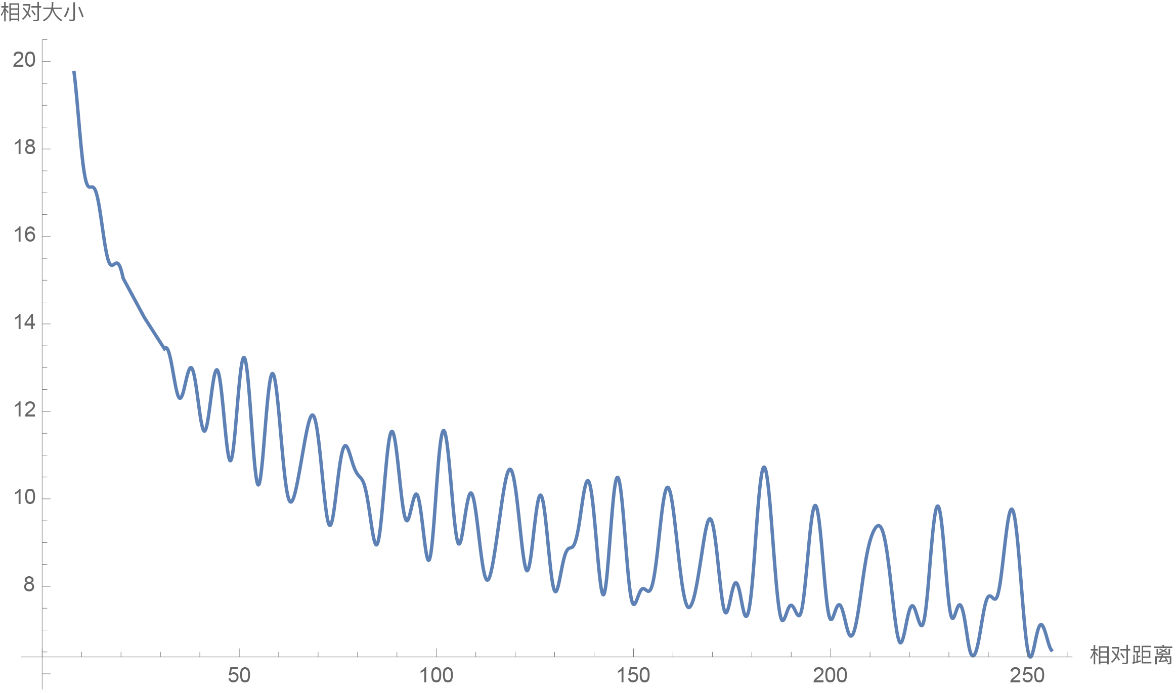
From the figure, we can see that as the relative distance increases, the inner product result shows a decaying trend. Therefore, choosing \theta_i = 10000^{-2i/d} indeed brings a certain degree of long-term decay. Of course, as mentioned in the previous article, this is not the only choice that can bring long-term decay; almost any smooth monotonic function would work. Here we simply followed the existing choice. The author also tried treating \theta_i as a trainable parameter initialized with 10000^{-2i/d}, but found that \theta_i did not update significantly after training for a while, so it was simply fixed to 10000^{-2i/d}.
Linear Scenarios
Finally, we point out that RoPE is currently the only relative position encoding that can be used for Linear Attention. This is because other relative position encodings are based on operations directly on the Attention matrix. However, Linear Attention does not calculate the Attention matrix explicitly, so such operations cannot be applied. Since RoPE implements relative position encoding via absolute position encoding, it does not require operating on the Attention matrix, making its application to Linear Attention possible.
For an introduction to Linear Attention, please refer to "Exploration of Linear Attention: Does Attention Need a Softmax?". The common form of Linear Attention is: Attention(\boldsymbol{Q},\boldsymbol{K},\boldsymbol{V})_i = \frac{\sum_{j=1}^n \text{sim}(\boldsymbol{q}_i, \boldsymbol{k}_j)\boldsymbol{v}_j}{\sum_{j=1}^n \text{sim}(\boldsymbol{q}_i, \boldsymbol{k}_j)} = \frac{\sum_{j=1}^n \phi(\boldsymbol{q}_i)^{\top} \varphi(\boldsymbol{k}_j)\boldsymbol{v}_j}{\sum_{j=1}^n \phi(\boldsymbol{q}_i)^{\top} \varphi(\boldsymbol{k}_j)} where \phi, \varphi are activation functions with non-negative ranges. Since Linear Attention is also based on inner products, a natural idea is to insert RoPE into the inner product: \frac{\sum_{j=1}^n [\boldsymbol{\mathcal{R}}_i\phi(\boldsymbol{q}_i)]^{\top} [\boldsymbol{\mathcal{R}}_j\varphi(\boldsymbol{k}_j)]\boldsymbol{v}_j}{\sum_{j=1}^n [\boldsymbol{\mathcal{R}}_i\phi(\boldsymbol{q}_i)]^{\top} [\boldsymbol{\mathcal{R}}_j\varphi(\boldsymbol{k}_j)]} However, the problem is that the inner product [\boldsymbol{\mathcal{R}}_i\phi(\boldsymbol{q}_i)]^{\top} [\boldsymbol{\mathcal{R}}_j\varphi(\boldsymbol{k}_j)] could be negative. Thus, it is no longer a conventional probabilistic attention, and the denominator risks being zero, which might cause instability in optimization. Considering that \boldsymbol{\mathcal{R}}_i and \boldsymbol{\mathcal{R}}_j are orthogonal matrices that do not change the vector norm, we can discard the conventional probabilistic normalization requirement and use the following operation as a new type of Linear Attention: \frac{\sum_{j=1}^n [\boldsymbol{\mathcal{R}}_i\phi(\boldsymbol{q}_i)]^{\top} [\boldsymbol{\mathcal{R}}_j\varphi(\boldsymbol{k}_j)]\boldsymbol{v}_j}{\sum_{j=1}^n \phi(\boldsymbol{q}_i)^{\top} \varphi(\boldsymbol{k}_j)} That is, RoPE is only inserted into the numerator, while the denominator remains unchanged. This attention is no longer based on probability (the attention matrix no longer satisfies non-negative normalization), but in some sense, it is still a normalization scheme. Furthermore, there is no evidence that non-probabilistic attention is necessarily worse (for example, Nyströmformer does not strictly construct attention based on probability distributions). We tested this as one of the candidate schemes, and our preliminary experimental results show that such Linear Attention is also effective.
Additionally, in "Exploration of Linear Attention: Does Attention Need a Softmax?", the author proposed another Linear Attention scheme: \text{sim}(\boldsymbol{q}_i, \boldsymbol{k}_j) = 1 + \left( \frac{\boldsymbol{q}_i}{\Vert \boldsymbol{q}_i\Vert}\right)^{\top}\left(\frac{\boldsymbol{k}_j}{\Vert \boldsymbol{k}_j\Vert}\right). This does not rely on non-negativity, and since RoPE does not change the norm, it can be directly applied to this type of Linear Attention without altering its probabilistic meaning.
Model Release
The first version of the RoFormer model has been trained and open-sourced on GitHub:
Simply put, RoFormer is a WoBERT model where absolute position encoding is replaced by RoPE. Its structural comparison with other models is as follows:
| BERT | WoBERT | NEZHA | RoFormer | |
|---|---|---|---|---|
| Token Unit | Character | Word | Character | Word |
| Pos. Encoding | Absolute | Absolute | Classical Relative | RoPE |
For pre-training, based on WoBERT Plus, we adopted a method of alternating training with multiple lengths and batch sizes to allow the model to adapt to different training scenarios in advance:
| Stage | maxlen | batch size | Steps | Final loss | Final acc |
|---|---|---|---|---|---|
| 1 | 512 | 256 | 200k | 1.73 | 65.0% |
| 2 | 1536 | 256 | 12.5k | 1.61 | 66.8% |
| 3 | 256 | 256 | 120k | 1.75 | 64.6% |
| 4 | 128 | 512 | 80k | 1.83 | 63.4% |
| 5 | 1536 | 256 | 10k | 1.58 | 67.4% |
| 6 | 512 | 512 | 30k | 1.66 | 66.2% |
As seen from the table, increasing the sequence length actually improved the pre-training accuracy. This indirectly reflects RoFormer’s effectiveness in processing long-text semantics and demonstrates that RoPE has good extrapolation capabilities. On short-text tasks, RoFormer performs similarly to WoBERT. The main feature of RoFormer is its ability to directly handle texts of arbitrary length. Below are our experimental results on the CAIL2019-SCM task:
| Validation Set | Test Set | |
|---|---|---|
| BERT-512 | 64.13% | 67.77% |
| WoBERT-512 | 64.07% | 68.10% |
| RoFormer-512 | 64.13% | 68.29% |
| RoFormer-1024 | 66.07% | 69.79% |
The parameter after the hyphen indicates the maxlen truncation during fine-tuning. It can be seen that RoFormer indeed handles long-text semantics better. Regarding hardware requirements, on a card with 24G VRAM, running maxlen=1024 with a batch_size of 8 or more is possible. Currently, in Chinese tasks, this is the only one the author found suitable for testing long-text capabilities. Readers are welcome to test or recommend other evaluation tasks.
Of course, although RoFormer can theoretically handle sequences of any length, it currently still has quadratic complexity. We are also training a RoFormer model based on Linear Attention, which will be released after experiments are completed. Please stay tuned.
(Note: RoPE and RoFormer have been compiled into the paper "RoFormer: Enhanced Transformer with Rotary Position Embedding" and submitted to Arxiv. Feel free to use and cite it!)
Summary
This article introduced our self-developed Rotary Position Embedding (RoPE) and the corresponding pre-trained model RoFormer. Theoretically, RoPE shares some commonalities with Sinusoidal position encoding, but RoPE does not rely on Taylor expansion and is more rigorous and interpretable. From the results of the pre-trained RoFormer model, RoPE shows good extrapolation and demonstrates superior long-text processing capabilities when applied to Transformers. Furthermore, RoPE is currently the only relative position encoding that can be used for Linear Attention.