Today, I would like to introduce a paper from 1962 titled "Computer Multiplication and Division Using Binary Logarithms", authored by John N. Mitchell. In this paper, he proposed a quite interesting algorithm: in binary, multiplication of two numbers can be approximated entirely through addition, with a maximum error not exceeding 1/9. The entire algorithm is quite ingenious, and even more interestingly, it has a very concise programming implementation that is truly striking. However, I found that there are surprisingly few web pages introducing this algorithm, so I will present it here.
Do you think this is just an obsolete relic? You would be wrong. Not long ago, someone used it to publish a paper at NeurIPS 2020! So, are you sure you don’t want to learn about it?
Fast Logarithms and Exponentials
When talking about turning multiplication into addition, one naturally thinks of logarithms and exponentials, namely: pq = a^s, \quad s = \log_a p + \log_a q This article is based on binary, so a=2. The problem is that while the above equation indeed converts multiplication to addition, calculating the logarithms \log_2 p, \log_2 q and the resulting exponential 2^s is not an easy task. Therefore, to use this identity for multiplication, the key lies in implementing fast logarithm and exponential operations.
For a non-negative decimal number p, let us assume its binary representation is: z_n z_{n-1} \cdots z_1 z_0 . z_{-1} z_{-2} \cdots z_{-(m-1)} z_{-m} where z_n = 1 and each z_i \in \{0,1\}. Then we have: p = 2^n + \sum_{i=-m}^{n-1} z_i 2^i = 2^n\left(1 + \sum_{i=-m}^{n-1} z_i 2^{i-n}\right) Let x = \sum\limits_{i=-m}^{n-1} z_i 2^{i-n}. We get: \log_2 p = n + \log_2\left(1 + x\right) Here, Mitchell made a quite bold and beautiful approximation, which is \log_2(1 + x) \approx x (we will perform an error analysis later). Thus, we obtain: \log_2 p \approx n + x What is so wonderful about this result? First, n is an integer, equal to the number of digits in the integer part of the binary representation of p minus 1; its binary conversion is naturally an integer. What about x? According to the definition of x, it is not hard to see that the binary representation of x is actually: 0 . z_{n-1} \cdots z_1 z_0 z_{-1} z_{-2} \cdots z_{-(m-1)} z_{-m} In other words, x is simply the fractional part of the approximation, and its binary representation is just a simple transformation (a decimal point shift) of the binary representation of p.
In summary, we obtain the Mitchell approximation algorithm for logarithms:
1. Input a decimal number p;
2. Convert p to a binary number z_n z_{n-1} \cdots z_1 z_0 . z_{-1} z_{-2} \cdots z_{-(m-1)} z_{-m}, where z_n=1;
3. Convert n to a binary number y_k y_{k-1} \cdots y_1 y_0;
4. Then the binary approximation of \log_2 p is y_k y_{k-1} \cdots y_1 y_0 . z_{n-1} \cdots z_1 z_0 z_{-1} z_{-2} \cdots z_{-(m-1)} z_{-m}.
By reversing the above process, we get the Mitchell approximation algorithm for exponentials:
1. Input a binary number z_n z_{n-1} \cdots z_1 z_0 . z_{-1} z_{-2} \cdots z_{-(m-1)} z_{-m};
2. Convert z_n z_{n-1} \cdots z_1 z_0 to a decimal number n;
3. Then the binary approximation of its exponential is 1 z_{-1} z_{-2} \cdots z_{-(n-1)} z_{-n} . z_{-(n+1)} z_{-(n+2)}\cdots z_{-(m-1)} z_{-m};
4. Convert the result to decimal.
So, in binary, the approximate calculation of logarithms and exponentials is just a matter of counting and concatenation! Isn’t it amazing?
A Multiplication Example
With the fast (approximate) logarithm and exponential algorithms, we can perform multiplication. Let’s use this approach to calculate a specific example to deepen our understanding of the process.
We want to calculate 12.3 \times 4.56. The calculation process is shown in the table below (the approximate exponential is calculated based on the result of the sum):
| p, q (Decimal) | 12.3 | 4.56 |
|---|---|---|
| p, q (Binary) | 1100.0100110 | 100.1000111 |
| n (Decimal) | 3 | 2 |
| n (Binary) | 11 | 10 |
| x (Binary) | 0.1000100110 | 0.001000111 |
| n+x (Binary) | 11.1000100110 | 10.001000111 |
| Sum (Binary) | 101.10101101 | |
| n (Binary) | 101 | |
| n (Decimal) | 5 | |
| x (Binary) | 0.10101101 | |
| Approx. Exp (Binary) | 110101.101 | |
| Approx. Exp (Decimal) | 53.625 | |
| Exact Product (Decimal) | 56.088 | |
| Relative Error (Decimal) | 4.39% | |
Note that the binary representations of p and q are infinite repeating decimals; here they are truncated to a finite number of bits. If the exact binary representation were preserved, the final result would be 53.68, which is not much different from the 53.625 in the table. As can be seen, the main computational load of the entire process consists of two parts: summation, and the conversion between decimal and binary. However, although the conversion between decimal and binary is a computationally intensive operation for humans, for computers, which store data in binary, we can consider the conversion cost to be negligible. Or rather, as long as we still output in decimal, this part of the calculation is inevitable regardless of the algorithm, so we do not include it in the algorithm’s complexity. Therefore, the computational load of the entire algorithm is just the summation step, achieving the (approximate) conversion of multiplication into addition.
Miraculous C++ Implementation
Even better, the above process has a very simple C++ implementation, as follows:
#include<stdio.h>

int main() {
    float a = 12.3f;
    float b = 4.56f;
    int c = *(int*)&a + *(int*)&b - 0x3f800000;
    printf("Approximate result: %f\n", *(float*)&c);
    printf("Exact result: %f\n", a * b);
    return 0;
}
Friends without a C++ compilation environment can find an online C++ runner to test the results. Even those who do not understand C++ (like myself) can probably sense that this code roughly converts the operation into the addition of two numbers and the subtraction of a constant. How can this achieve multiplication? Some readers might also ask if this can be written in Python.
First, the answer to the latter question is no, because Python’s data types are highly encapsulated. The feasibility of the C++ code above lies in the IEEE 754 representation of floating-point numbers: a decimal floating-point number is first converted to binary, then normalized into scientific notation, and finally stored in a specific structure. Specifically, IEEE 754 uses 32 bits to represent a float, where 1 bit is for the sign (0 for positive), 8 bits for the exponent of the scientific notation, and 23 bits for the fraction. Taking 9.75 as an example, its binary is 1001.11, which in scientific notation is 1.00111 \times 2^3. Note that for the exponent part, we need to add an offset of 127, so the exponent 3 is actually stored as 130 (binary 10000010). For the mantissa part 1.00111, since the first digit is always 1, only 0.00111 needs to be stored. Thus, the representation of 9.75 is:
| Sign | Exponent | Fraction |
|---|---|---|
| 0 | 10000010 | 0011100 00000000 00000000 |
Knowing the IEEE 754 representation, we can understand the code.
*(int*)&a and *(int*)&b actually
extract the IEEE 754 representations of a and b and
treat them as ordinary integers. Adding them together corresponds
exactly to the addition of the Mitchell-approximated logarithms.
However, the exponent part will have an extra offset, so the total
offset must be subtracted. Since the offset is 127 and there are 23 bits
following it, subtracting the offset is equivalent to subtracting the
constant 127 \times 2^{23}, which is
0x3f800000 in hexadecimal. Finally, the result of the
addition and subtraction is restored to a floating-point number.
(Note: I do not actually understand C++; the above explanation is pieced together. If there are inaccuracies, please point them out.)
Analysis of Maximum Error
The title states that the error of this algorithm does not exceed 1/9. We will now prove this. The proof is best understood by converting everything back to decimal. The Mitchell approximation essentially uses the following approximations: \log_2 2^n(1+x) \approx n + x, \quad 2^{n+x} \approx 2^n(1+x) where n is an integer and x \in [0, 1). The error analysis starts from these two approximations.
Suppose two numbers are p = 2^{n_1}(1 + x_1) and q = 2^{n_2}(1 + x_2). According to the approximation, \log_2 p + \log_2 q \approx n_1 + n_2 + x_1 + x_2. There are two cases to discuss:
Case 1: x_1 + x_2 < 1. The approximate exponential result is 2^{n_1 + n_2}(1 + x_1 + x_2). The approximation ratio is: \frac{2^{n_1 + n_2}(1 + x_1 + x_2)}{2^{n_1}(1 + x_1) \times 2^{n_2}(1 + x_2)} = \frac{1 + x_1 + x_2}{1 + x_1 + x_2 + x_1 x_2}
Case 2: x_1 + x_2 \geq 1. In this case, the approximate exponential result is 2^{n_1 + n_2 + 1}(x_1 + x_2 + 1 - 1) = 2^{n_1 + n_2 + 1}(x_1 + x_2), so the approximation ratio is: \frac{2^{n_1 + n_2 + 1}(x_1 + x_2)}{2^{n_1}(1 + x_1) \times 2^{n_2}(1 + x_2)} = \frac{2(x_1 + x_2)}{1 + x_1 + x_2 + x_1 x_2}
It can be proven step-by-step that the minimum value for both cases occurs at x_1 = x_2 = 0.5, where the result is 8/9. Thus, the maximum relative error is 1/9 (if division is converted to subtraction, the maximum error is 12.5\%). Since the formal proof is somewhat tedious, we will not repeat it here but instead use software to plot the contour map. It can be seen that the error is largest at the center:
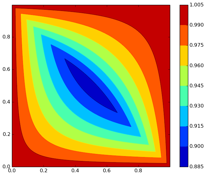
Plotting code:
import numpy as np
import matplotlib.pyplot as plt

x = np.arange(0, 1, 0.001)
y = np.arange(0, 1, 0.001)

X, Y = np.meshgrid(x, y)
Z1 = (1 + X + Y) / (1 + X + Y + X * Y)
Z2 = 2 * (X + Y) / (1 + X + Y + X * Y)
Z = (X + Y < 1) * Z1 + (X + Y >= 1) * Z2
plt.figure(figsize=(7, 6))
contourf = plt.contourf(X, Y, Z)
plt.contour(X, Y, Z)
plt.colorbar(contourf)
plt.show()
In fact, this error essentially depends on the degree of approximation of \log_2(1 + x) \approx x. We know that x is the first-order Taylor expansion of the natural logarithm \ln(1 + x), and e = 2.71828\dots is closer to 3. Therefore, if computers used base-3, this algorithm would have higher average precision. Indeed, some theoretical analyses suggest that for computers, base-e would be ideal, and 3 is closer to e than 2. Thus, ternary computers would be superior to binary computers in many aspects. Both China and the former Soviet Union studied ternary computers, but because binary is easier to implement, binary computers dominate today.
Moving into Deep Learning
This concludes the introduction to the Mitchell approximation. Readers might be puzzled: shouldn’t this be part of computer fundamentals or data structures? Why study it? Can it have any application in deep learning?
I studied it for two reasons: first, it is indeed beautiful and worth learning; second, it can actually be used in deep learning. In fact, I discovered it in a NeurIPS 2020 paper titled "Deep Neural Network Training without Multiplications". The paper verified on "ImageNet + ResNet50" that directly replacing multiplications in neural networks with the Mitchell approximation’s addition form results in only a slight decrease in accuracy, or even no decrease at all.
Of course, the authors’ current implementation only verifies that this replacement is acceptable in terms of effect; in terms of speed, it is actually slower. This is because, although theoretically replacing multiplication with approximate addition should increase speed, achieving this improvement requires optimization at the hardware level. Current standard multiplication is already optimized at the hardware level, so the authors provide a direction for future deep learning hardware optimization. Furthermore, the application of the Mitchell approximation in deep learning is not being discussed for the first time; a quick Google search reveals two other papers: "Efficient Mitchell’s Approximate Log Multipliers for Convolutional Neural Networks" and "Low-power implementation of Mitchell’s approximate logarithmic multiplication for convolutional neural networks".
Readers might be reminded of AdderNet, proposed by Huawei. Its purpose is indeed similar, but the method is quite different. AdderNet replaces the dot product in neural networks with l_1 distance, thereby removing multiplication; this paper modifies the implementation of multiplication to reduce the computational cost, allowing existing neural network operations to be preserved.
Old Wine in New Bottles
This article introduced the Mitchell approximation algorithm published in 1962. It is an approximate logarithm and exponential calculation, based on which we can convert multiplication into addition while maintaining a certain level of precision. It seems outdated, but by putting this "old wine in a new bottle," it became a paper at NeurIPS 2020.
So, what other "old wines" have you found that could be put into new bottles?
Reprinting: Please include the original link: https://kexue.fm/archives/7991
Further details on reprinting: Please refer to the Scientific Space FAQ.