Since SimCLR, work on unsupervised feature learning in Computer Vision (CV) has emerged in an endless stream, making it quite dazzling. Most of these works are based on contrastive learning, which involves constructing positive and negative samples in an appropriate way for classification learning. However, among many similar works, there are always some unconventional studies, such as Google’s BYOL and the recent SimSiam. They propose schemes that can complete feature learning relying only on positive samples, which is refreshing. But without the support of negative samples, why doesn’t the model degenerate (collapse) into a meaningless constant model? This is the most thought-provoking and memorable question in these two papers.
SimSiam provides an answer that many have praised, but I feel that SimSiam merely rephrased the problem rather than truly solving it. I believe that a significant reason for the success of models like SimSiam and GANs is the use of gradient-based optimizers (rather than other stronger or weaker optimizers). Therefore, any answer that does not incorporate optimization dynamics is incomplete. Here, I attempt to analyze why SimSiam does not degenerate from the perspective of dynamics.
SimSiam
Before looking at SimSiam, we can first look at BYOL, from the paper "Bootstrap your own latent: A new approach to self-supervised Learning". Its learning process is very simple: it maintains two encoders, Student and Teacher, where the Teacher is a moving average of the Student, and the Student in turn learns from the Teacher. It feels like "stepping on your own left foot with your right foot" to fly. The schematic is as follows:
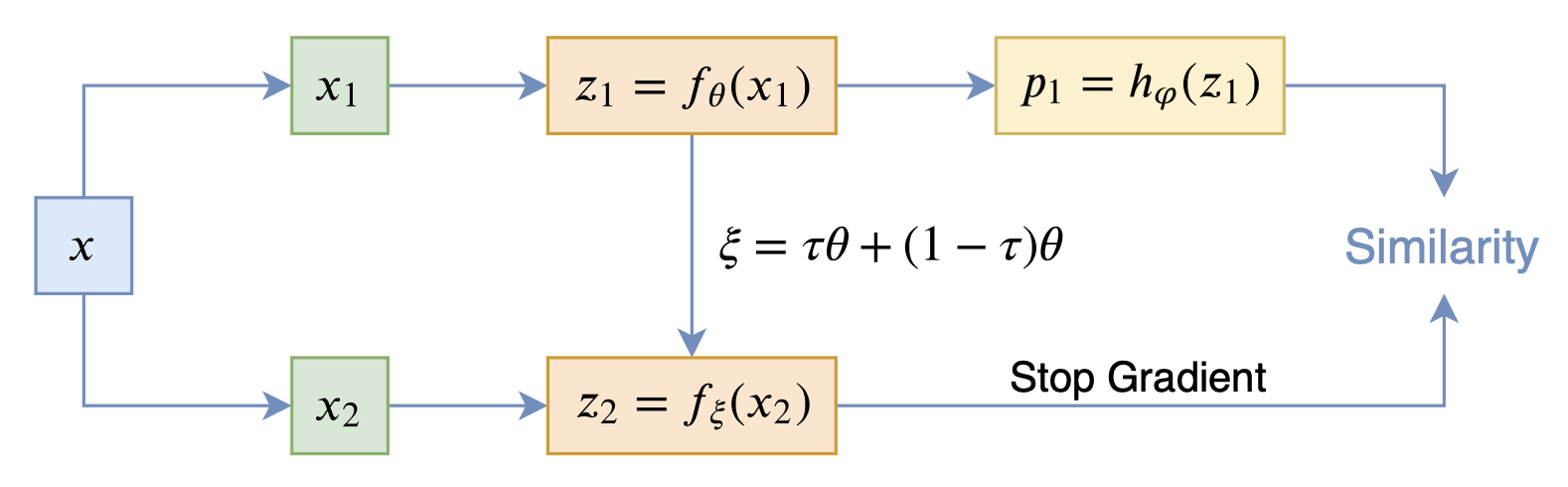
SimSiam comes from the paper "Exploring Simple Siamese Representation Learning". It is even simpler, directly removing the moving average of BYOL:
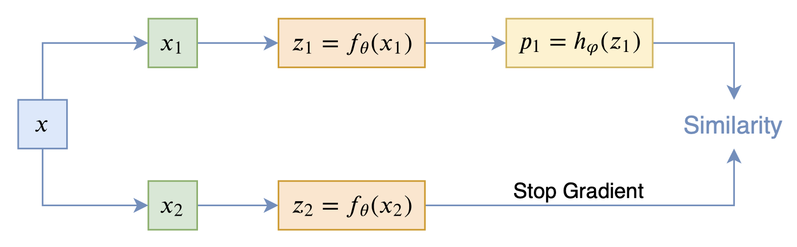
In fact, SimSiam is equivalent to setting the moving average
parameter \tau of BYOL to 0, which
shows that the moving average in BYOL is not essential. To find the key
parts of the algorithm, SimSiam also conducted many comparative
experiments, confirming that the stop_gradient operator and
the predictor module h_{\varphi}(z) are
key to SimSiam’s non-degeneration. To explain this phenomenon, SimSiam
proposed that the optimization process is actually equivalent to
alternating optimization of: \mathcal{L}(\theta, \eta)=\mathbb{E}_{x,
\mathcal{T}}\left[\left\Vert\mathcal{F}_{\theta}(\mathcal{T}(x))-\eta_{x}\right\Vert^2\right]\label{eq:simsiam}
where x represents training samples and
\mathcal{T} represents data
augmentation. There are already many interpretations of this part
online, and reading the original paper is not difficult, so I will not
expand on it in detail.
Dynamics Analysis
However, I believe that converting the understanding of the SimSiam algorithm into the understanding of the alternating optimization of \mathcal{L}(\theta, \eta) is just a change of wording and does not provide a substantial answer. Because obviously, \mathcal{L}(\theta, \eta) also has a degenerate solution: the model could simply make all \eta_{x} equal to the same vector, and then \mathcal{F}_{\theta} outputs the same constant vector. If you don’t answer why the alternating optimization of \mathcal{L}(\theta, \eta) does not degenerate, then you haven’t answered the question.
Below, I will list what I consider to be the key factors for SimSiam’s non-degeneration and use a simple example to show that answering the cause of non-degeneration needs to be combined with dynamics. Of course, my discourse in this part is also incomplete and perhaps even unrigorous; it is just a new perspective intended to stimulate further discussion.
Deep Image Prior
First of all, it was discovered long ago that a randomly initialized CNN model can be used directly to extract visual features, and the effect is not particularly bad. This conclusion can be traced back to the 2009 paper "What is the best multi-stage architecture for object recognition?". This can be understood as CNNs having a natural ability to process images. Later, this characteristic was given a sophisticated name, "Deep Image Prior," from the paper "Deep Image Prior". They conducted experiments showing that starting from a randomly initialized CNN model, tasks like image completion and denoising can be completed without any supervised learning, further confirming the characteristic that CNNs naturally possess image processing capabilities.
According to my understanding, "Deep Image Prior" stems from three points:
Image Continuity: This means that the image itself can be directly viewed as a continuous vector, without needing to learn an Embedding layer like in NLP. This means we can do many tasks using simple methods like "original image + K-nearest neighbors."
CNN Architecture Prior: This refers to the local perception design of CNNs, which indeed simulates the visual processing of the human eye well. Since the visual classification results we provide are also based on our human eyes, the two are consistent.
Good Initialization: This is not hard to understand. Even the best model with all-zero initialization probably won’t work. A previous article "Understanding Model Parameter Initialization Strategies from a Geometric Perspective" also briefly discussed initialization methods. From a geometric sense, mainstream initialization methods are a kind of approximate "orthogonal transformation," which can preserve the information of input features as much as possible.
Dynamics of Non-Degeneration
Again, the deep image prior means that a randomized CNN model is already a "not-so-bad" encoder. So what we need to do next can be summarized into two points: learn in a better direction, and do not degenerate toward a constant.
Learning in a better direction means designing some prior signals to allow the model to better integrate this prior knowledge. SimSiam, BYOL, etc., let the same image undergo two different data augmentations and then make the corresponding feature vectors as similar as possible. This is a good signal guidance, telling the model that simple transformations should not affect our visual understanding. In fact, this is one of the designs used by all contrastive learning methods.
The difference lies in the point of "not degenerating toward a
constant." General contrastive learning methods tell the model which
image features should not be similar by constructing negative samples,
thereby preventing the model from degenerating. However, SimSiam and
BYOL are different; they have no negative samples. In fact, they prevent
degeneration by decomposing the model’s optimization process into two
synchronized but differently paced modules. Taking SimSiam as an
example, its optimization objective can be written as: \mathcal{L}(\varphi, \theta)=\mathbb{E}_{x,
\mathcal{T}_1,\mathcal{T}_2}\Big[l\left(h_{\varphi}(f_{\theta}(\mathcal{T}_1(x))),
f_{\theta}(\mathcal{T}_2(x))\right)\Big] Then using gradient
descent to optimize, the corresponding dynamical equations are: \begin{aligned}
\frac{d\varphi}{dt} = - \frac{\partial\mathcal{L}}{\partial \varphi}
=& -\mathbb{E}_{x, \mathcal{T}_1,\mathcal{T}_2}\bigg[\frac{\partial
l}{\partial h}\frac{\partial h}{\partial \varphi}\bigg]\\
\frac{d\theta}{dt} = - \frac{\partial\mathcal{L}}{\partial \theta}
=& -\mathbb{E}_{x, \mathcal{T}_1,\mathcal{T}_2}\bigg[\frac{\partial
l}{\partial h}\frac{\partial h}{\partial f}\frac{\partial f}{\partial
\theta} \color{blue}{\,+\underbrace{\frac{\partial l}{\partial
f}\frac{\partial f}{\partial
\theta}}_{\begin{aligned}\text{SimSiam}\\\text{removed
this}\end{aligned}}}\bigg]
\end{aligned} The above equation indicates the difference brought
by the presence or absence of the stop_gradient operator.
Simply put, if the stop_gradient operator is added, then
\frac{d\theta}{dt} lacks the second
term. In this case, both \frac{d\varphi}{dt} and \frac{d\theta}{dt} share the factor \frac{\partial l}{\partial h}. Since h_{\varphi} is closer to the output layer and
the initialized f_{\theta} is also a
decent encoder, at the start of learning, h_{\varphi} will be optimized faster, while
parts closer to the input layer optimize slower. That is to say, \frac{d\varphi}{dt} is the fast dynamics
part, and \frac{d\theta}{dt} is the
slow dynamics part. Relatively speaking, \frac{d\varphi}{dt} will converge to 0 more
quickly. This means \frac{\partial l}{\partial
h} will quickly become very small. Since \frac{d\theta}{dt} also contains the \frac{\partial l}{\partial h} term, \frac{d\theta}{dt} becomes small along with
it. Before it can degenerate, the force driving it to degenerate has
become negligible, so it won’t degenerate. Conversely, if there is the
second term \frac{\partial l}{\partial
f}\frac{\partial f}{\partial \theta} (whether it’s added back or
only it is kept), it is equivalent to adding a "fast track," making it a
fast term. Even if \frac{\partial l}{\partial
h}=0, because the second term exists, it will continue to drive
it toward degeneration.
Let’s take a simple specific example. Consider: l = \frac{1}{2}(\varphi\theta - \theta)^2 For simplicity, \varphi, \theta are scalars. The corresponding dynamical equations are: \frac{d\varphi}{dt}=-(\varphi\theta - \theta)\theta, \quad\frac{d\theta}{dt}=-(\varphi\theta - \theta) \varphi \color{blue}{+ \underbrace{(\varphi\theta - \theta)}_{\begin{aligned}\text{SimSiam}\theta\\ \text{removed this}\end{aligned}}} Suppose \varphi(0)=0.6, \theta(0)=0.1 (chosen arbitrarily). The evolution of both is:
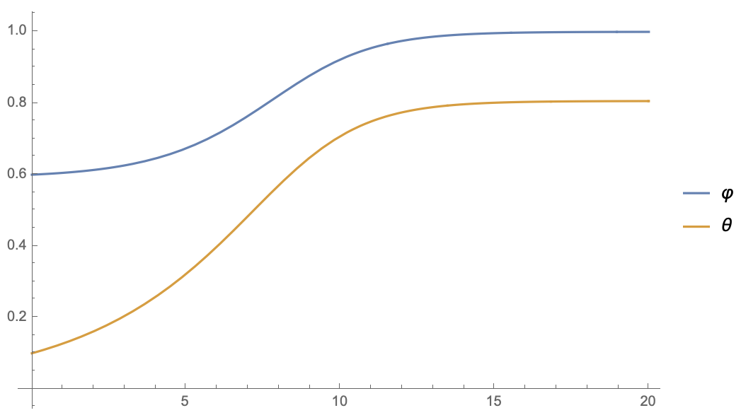
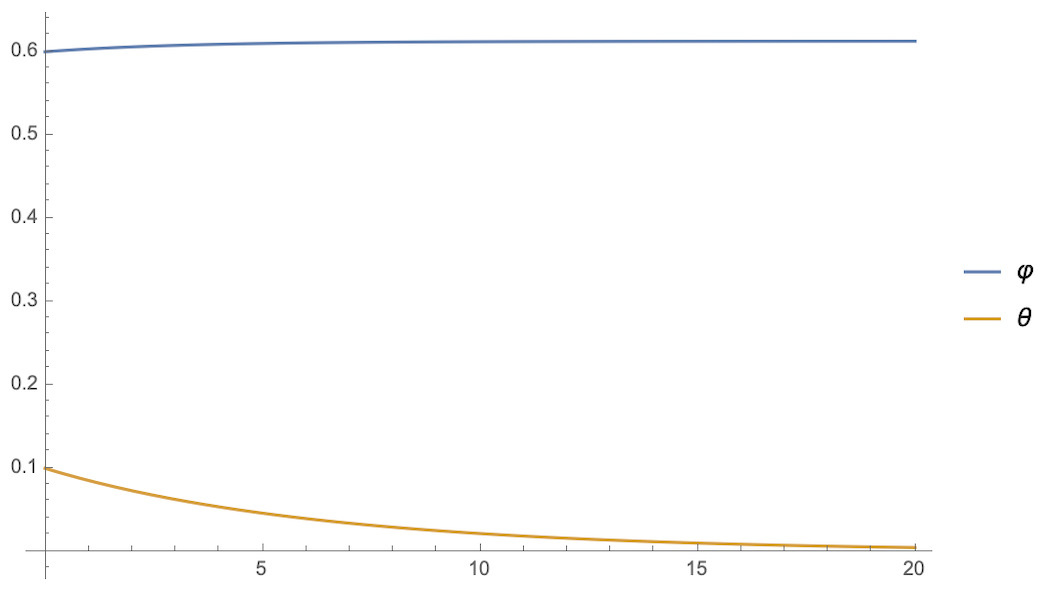
As can be seen, after stopping the gradient of the second \theta, the equations for \varphi and \theta are quite consistent; \varphi quickly tends to 1, while \theta stabilizes at a non-zero value (meaning no degeneration). Conversely, if the second term of \frac{d\theta}{dt} is added, or if only the second term is kept, the result is that \theta quickly tends to 0, and \varphi cannot tend to 1. This means the dominance is taken over by \theta.
This example itself isn’t highly persuasive, but it simply reveals the changes in dynamics:
The introduction of the predictor (\varphi) divides the model’s dynamics into two major parts. The introduction of the
stop_gradientoperator makes the dynamics of the encoder part (\theta) slower and enhances the synchronization between the encoder and the predictor. In this way, the predictor fits the target with "lightning speed," so that the optimization process stops before the encoder has time to degenerate.
Looking at the Approximate Expansion
Of course, there are thousands of interpretations, all of which are "hindsight." The truly great ones are the discoverers; at most, we are just riding the coattails. Let me ride a bit more by sharing another perspective I have on SimSiam. As mentioned at the beginning, the SimSiam paper proposed explaining SimSiam through the alternating optimization of objective \eqref{eq:simsiam}. This perspective starts from objective \eqref{eq:simsiam} and delves further into the reasons for its non-degeneration.
If \theta is fixed, then for
objective \eqref{eq:simsiam}, it is
easy to solve for the optimal value of \eta_x: \eta_x=\mathbb{E}_{\mathcal{T}}\left[\mathcal{F}_{\theta}(\mathcal{T}(x))\right]
Substituting this into \eqref{eq:simsiam}, we get the optimization
objective as: \mathcal{L}(\theta)=\mathbb{E}_{x,
\mathcal{T}}\bigg[\Big\Vert\mathcal{F}_{\theta}(\mathcal{T}(x))-\mathbb{E}_{\mathcal{T}}\left[\mathcal{F}_{\theta}(\mathcal{T}(x))\right]\Big\Vert^2\bigg]
We assume that \mathcal{T}(x)-x is a
"small" vector. Then, performing a first-order expansion at x gives: \mathcal{L}(\theta)\approx\mathbb{E}_{x,
\mathcal{T}}\bigg[\left\Vert\frac{\partial
\mathcal{F}_{\theta}(x)}{\partial
x}\big(\mathcal{T}(x)-\bar{x}\big)\right\Vert^2\bigg]\label{eq:em-sim}
where \bar{x}=\mathbb{E}_{\mathcal{T}}\left[\mathcal{T}(x)\right]
is the average result of the same image under all data augmentation
methods. Note that it is usually not equal to x. Similarly, if it were SimSiam without
stop_gradient or a predictor, the loss function would be
approximately: \mathcal{L}(\theta)\approx\mathbb{E}_{x,
\mathcal{T}_1, \mathcal{T}_2}\bigg[\left\Vert\frac{\partial
\mathcal{F}_{\theta}(x)}{\partial
x}\big(\mathcal{T}_2(x)-\mathcal{T}_1(x)\big)\right\Vert^2\bigg]\label{eq:em-sim-2}
In equation \eqref{eq:em-sim}, each
\mathcal{T}(x) is subtracted by \bar{x}. It can be proven that this choice
minimizes the loss function. In equation \eqref{eq:em-sim-2}, each \mathcal{T}_1(x) is subtracted by another
augmentation result \mathcal{T}_2(x),
which causes both the loss function itself and the variance of the
estimate to increase significantly.
Does this mean that the reason why not adding
stop_gradient or a predictor fails is that its loss
function and variance are too large? Note that under the first-order
approximation, \eta_x \approx
\mathcal{F}_{\theta}(\bar{x}). If the optimization objective were
changed to: \mathcal{L}(\theta)=\mathbb{E}_{x,
\mathcal{T}}\bigg[\Big\Vert\mathcal{F}_{\theta}(\mathcal{T}(x))-\mathcal{F}_{\theta}(\bar{x})\Big\Vert^2\bigg]
would it then not degenerate? I have not verified this and do not know.
Readers currently researching related content might want to verify it.
This also leads to a related question: for an encoder trained this way,
is it better to use \mathcal{F}_{\theta}(x) or \mathcal{F}_{\theta}(\bar{x}) as the
feature?
Of course, the discussion in this section is based on the assumption that "\mathcal{T}(x)-x is a small vector." If this does not hold, then this section is for naught.
Summary
This article attempts to provide my understanding of why the BYOL and SimSiam algorithms do not degenerate from a dynamics perspective. Unfortunately, halfway through writing, I realized that some analyses I had conceived in my mind could not be reconciled, so I deleted some content and added a new perspective, trying to ensure the article didn’t "end in a mess." As for seeking perfection, that’s out of the question. Consider this a shared note; if there are any inaccuracies, I hope readers will be kind enough to correct them.
Original Address: https://kexue.fm/archives/7980