As is widely known, current mainstream BERT models can handle a maximum of 512 tokens. The fundamental cause of this bottleneck is that BERT utilizes absolute position embeddings trained from random initialization. Generally, the maximum position is set to 512; thus, it can handle at most 512 tokens, as there are no position embeddings available for any subsequent parts. Of course, another significant reason is the \mathcal{O}(n^2) complexity of the Attention mechanism, which leads to a massive increase in memory usage for long sequences, making fine-tuning impossible on standard GPUs.
This article primarily addresses the former cause. Assuming sufficient memory is available, we explore how to simply modify a BERT model with a current maximum length of 512 so that it can directly process longer text. The main idea is to hierarchically decompose the pre-trained absolute position embeddings, allowing them to be extended to longer positions.
Position Embeddings
BERT uses trained absolute position embeddings. This method is simple and direct, and its performance is quite good. However, because each position vector is learned by the model itself, we cannot infer the embedding vectors for other positions, which results in a length limit.
A mainstream approach to solving this problem is to switch to relative position embeddings. This is a viable method; for instance, Huawei’s NEZHA model is a BERT variant that uses relative position embeddings. Relative position embeddings typically truncate the position difference so that the relative positions to be processed fall within a finite range, thus making them independent of the sequence length. However, relative position embeddings are not a perfect solution. First, relative position embeddings like those in NEZHA increase the computational load (though T5’s implementation does not). Second, Linear Attention cannot use relative position embeddings, meaning they are not sufficiently universal.
Readers might recall that "Attention is All You Need" proposed a Sinusoidal absolute position embedding using \sin and \cos. Wouldn’t using that directly remove the length limit? Theoretically, yes, but the problem is that there are currently no open-source models using Sinusoidal position embeddings. Do we really have to train one from scratch? That is clearly unrealistic.
Hierarchical Decomposition
Therefore, given limited resources, the most ideal solution is to find a way to extend the trained BERT position embeddings without retraining the model. Below, I present a hierarchical decomposition scheme I devised.
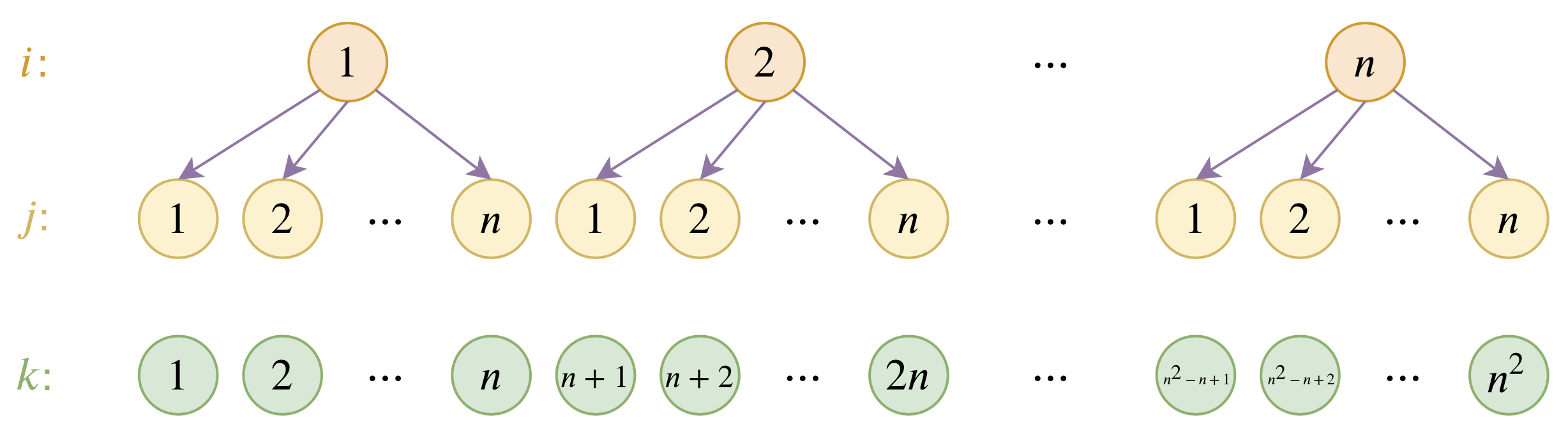
Specifically, assume the pre-trained absolute position embedding vectors are \boldsymbol{p}_1, \boldsymbol{p}_2, \cdots, \boldsymbol{p}_n. We hope to construct a new set of embedding vectors \boldsymbol{q}_1, \boldsymbol{q}_2, \cdots, \boldsymbol{q}_m based on these, where m > n. To this end, we set: \boldsymbol{q}_{(i-1)\times n + j} = \alpha \boldsymbol{u}_i + (1 - \alpha) \boldsymbol{u}_j \label{eq:decomposition} where \alpha \in (0, 1) and \alpha \neq 0.5 is a hyperparameter, and \boldsymbol{u}_1, \boldsymbol{u}_2, \cdots, \boldsymbol{u}_n are the "basis" for this set of position embeddings. The meaning of this representation is clear: the position (i - 1) \times n + j is hierarchically represented as (i, j), where the position embeddings corresponding to i and j are \alpha \boldsymbol{u}_i and (1 - \alpha) \boldsymbol{u}_j respectively, and the final embedding vector for (i - 1) \times n + j is the superposition of the two. The requirement \alpha \neq 0.5 is to distinguish between the two different cases (i, j) and (j, i).
We want the position vectors to remain the same as the original ones when the index does not exceed n, so as to be compatible with the pre-trained model. In other words, we want \boldsymbol{q}_1 = \boldsymbol{p}_1, \boldsymbol{q}_2 = \boldsymbol{p}_2, \cdots, \boldsymbol{q}_n = \boldsymbol{p}_n. From this, we can derive each \boldsymbol{u}_i: \boldsymbol{u}_i = \frac{\boldsymbol{p}_i - \alpha\boldsymbol{p}_1}{1 - \alpha}, \quad i = 1, 2, \cdots, n In this way, our parameters are still \boldsymbol{p}_1, \boldsymbol{p}_2, \cdots, \boldsymbol{p}_n, but we can represent embeddings for n^2 positions, and the first n position embeddings are compatible with the original model.
Self-Analysis
In fact, after understanding it, readers might feel that this decomposition doesn’t have much technical depth—it’s just a result of pure intuition. And indeed, it is.
As for why I think this works? First, because the hierarchical decomposition is highly interpretable, we can expect our results to have a certain degree of extrapolation capability; at least for positions greater than n, it serves as a decent initialization. Second, the experiments in the next section validate it—after all, experiments are the only standard for proving a trick’s effectiveness. Essentially, what we are doing is very simple: constructing an extension scheme for position embeddings that is compatible with the first n original embeddings and can extrapolate to more positions, leaving the rest for the model to adapt to. There are surely infinite ways to do this; I simply chose one that I found relatively interpretable, providing a possibility rather than the optimal or a guaranteed solution.
Furthermore, regarding the selection of \alpha, my default choice is \alpha = 0.4. Theoretically, any \alpha \in (0, 1) with \alpha \neq 0.5 holds, but from a practical standpoint, I suggest choosing a value where 0 < \alpha < 0.5. Since we rarely encounter sequences tens of thousands of tokens long—for a personal GPU, being able to handle 2048 is already quite "luxurious"—if n=512, this means i = 1, 2, 3, 4 while j = 1, 2, \cdots, 512. If \alpha > 0.5, then according to the decomposition formula [eq:decomposition], \alpha \boldsymbol{u}_i would dominate. Consequently, the differences between position embeddings would decrease (because there are only 4 candidates for i), making it harder for the model to distinguish between positions and leading to slower convergence. If \alpha < 0.5, then (1-\alpha) \boldsymbol{u}_j dominates, providing better discriminability for position embeddings (as there are 512 candidates for j), and the model converges faster.
Practical Testing
In summary, we can extend BERT’s absolute position embeddings at
almost zero cost, allowing the maximum length to reach n^2 = 512^2 = 262,144 \approx 260,000! This
should definitely satisfy our needs. This modification is already built
into bert4keras >= 0.9.5. Users only need to pass the
parameter hierarchical_position=True in
build_transformer_model to enable it. True can
also be replaced with a float between 0 and 1, representing the value of
\alpha mentioned above; when
True, the default is \alpha=0.4.
# Example usage in bert4keras
model = build_transformer_model(
    config_path,
    checkpoint_path,
    hierarchical_position=True
)
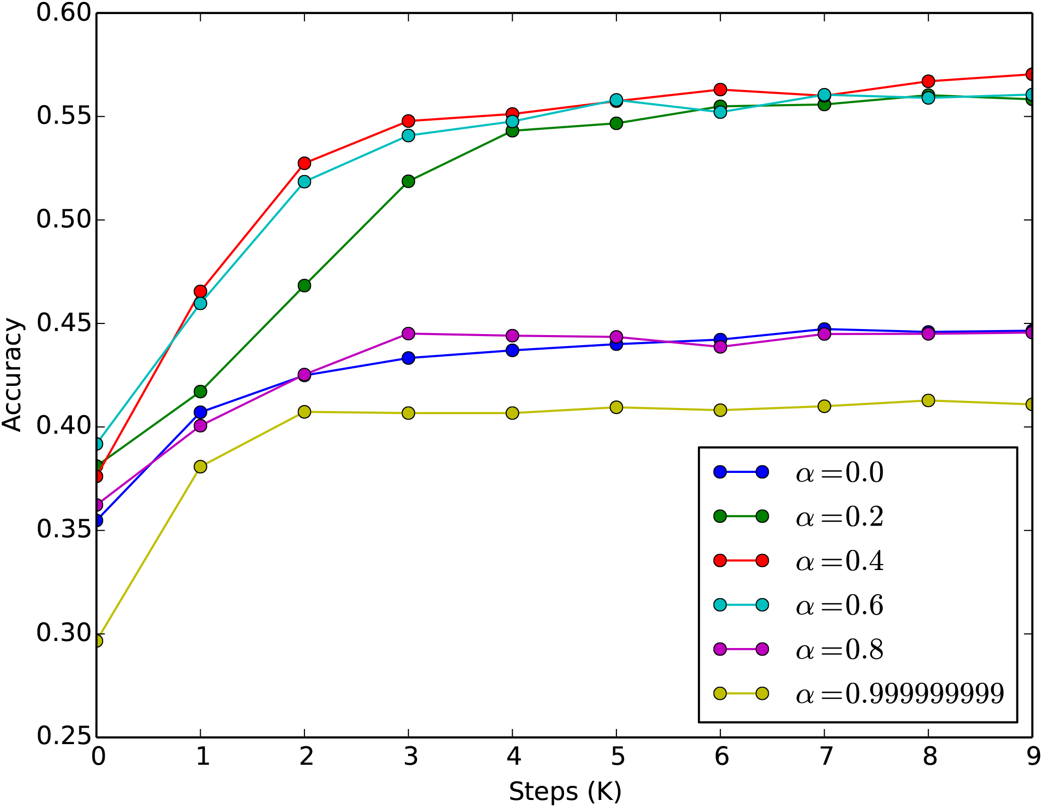
Regarding the results, I first tested the MLM task. I set the maximum length directly to 1536 and loaded the pre-trained RoBERTa weights. I found that the MLM accuracy was around 38% (if truncated to 512, it is about 55%). After fine-tuning, the accuracy quickly recovered to over 55% (in about 3000 steps). This result indicates that the position embeddings extended this way are effective for the MLM task. If you have spare computing power, it is likely beneficial to continue pre-training under MLM for a while before performing other tasks. Simultaneously, we experimented with different \alpha values, showing that \alpha=0.4 is indeed a good default, as shown in the figure below.
Then, I tested two long-text classification problems, setting the
lengths to 512 and 1024 respectively, and fine-tuned with other
parameters unchanged (direct fine-tuning, without prior MLM continued
pre-training). In one dataset, the results showed no significant change;
in the other, the 1024-length model outperformed the 512-length model by
about 0.5% on the validation set. This again demonstrates that the
hierarchical decomposition of position embeddings proposed in this
article works. So, if you have a GPU with enough memory, feel free to
give it a try, especially for long-text sequence labeling tasks, which I
suspect would be quite suitable. In bert4keras, it’s just
one extra line of code—if there’s an improvement, you’ve gained; if not,
you haven’t wasted much effort. I welcome everyone to report their own
test results.
Finally, here is a reference table for the maximum length and maximum batch size during the training phase (RoBERTa Base version, 24G TITAN RTX):
| Sequence Length | Batch Size |
|---|---|
| 512 | 22 |
| 1024 | 9 |
| 1536 | 5 |
From this table, we can see that when the sequence length doubles, the memory usage roughly doubles (slightly more), which seems different from the legendary \mathcal{O}(n^2) complexity. In fact, \mathcal{O}(n^2) is targeted at sufficiently long sequences—"sufficiently long" meaning thousands or tens of thousands. For sequences not exceeding 2048, BERT’s complexity is still nearly linear. Therefore, in such scenarios, using "BERT + extended position embeddings" is much more convenient than designs like "Sentence Splitting + BERT + LSTM".
Summary
This article shares a hierarchical decomposition-based extension scheme for position embeddings. Through this extension, BERT can theoretically process text up to 260,000 tokens in length. As long as there is enough memory, there is no long text that BERT cannot handle.
So, have you prepared your memory?
Original Address: https://kexue.fm/archives/7947
For more details on reprinting, please refer to: Scientific Space FAQ