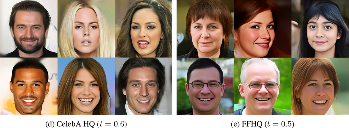
Yesterday morning, while doing my daily browse of arXiv, I was shocked by a newly released paper! The paper is titled "NVAE: A Deep Hierarchical Variational Autoencoder". As the name suggests, it is an improvement on VAE, proposing a new model called NVAE. To be honest, when I clicked on it, I didn’t have high hopes because I consider myself to have a certain understanding of VAEs and felt that their capacity for generative modeling was ultimately limited. However, when I opened the paper, the visual style presented was like this:
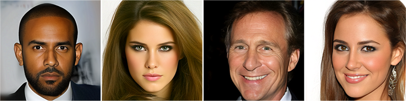
My first reaction was:
W!T!F! Is this really generated by a VAE? Is this still the VAE I know? It seems my understanding of VAE was too shallow; I can never say VAE-generated images are blurry again...
But after looking at the authors’ affiliation—NVIDIA—it became somewhat understandable. In recent years, many might have noticed that NVIDIA usually releases a breakthrough in generative models toward the end of the year: PGGAN in late 2017, StyleGAN in late 2018, and StyleGAN2 in late 2019. This year, they seem to be ahead of schedule and more active, as they just released a method called ADA last month, which pushed Cifar-10 generation to a new height, and now comes NVAE.
So, what is so special about NVAE that allows it to achieve such a leap in VAE generation quality?
VAE Review
A careful reader might observe:
It still looks a bit fake; the faces are too smooth, as if they’ve been airbrushed, and it’s not quite as good as StyleGAN yet...
Yes, that critique is not wrong; the generative artifacts are still quite noticeable. But if you aren’t shocked, it’s likely because you haven’t seen previous VAE generation results. The typical VAE generation style looks like this:
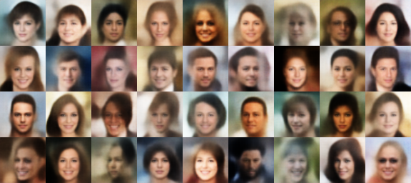
So, do you still think this isn’t a breakthrough?
What limited the expressive power of (previous) VAEs? And where did this breakthrough come from? Let’s continue.
Basic Introduction
VAE, or Variational Auto-Encoder, has been introduced in many articles on this blog. You can find many related posts by searching for "Variational Autoencoder" in the search bar. Here is a brief review and analysis.
In my derivation of VAE, we start with a set of samples representing a real (but unknown) distribution \tilde{p}(x). We then construct a parameterized posterior distribution p(z|x), and the two form a joint distribution p(x,z)=\tilde{p}(x)p(z|x). Next, we define a prior distribution q(z) and a generative distribution q(x|z), forming another joint distribution q(x,z)=q(z)q(x|z). Finally, our goal is to make p(x,z) and q(x,z) close to each other, so we optimize the KL divergence between them:
\begin{aligned} KL\big(p(x,z)\big\Vert q(x,z)\big) &= \iint p(x,z)\log \frac{p(x,z)}{q(x,z)} dzdx \\ &= \mathbb{E}_{x\sim \tilde{p}(x)} \Big[\mathbb{E}_{z\sim p(z|x)}\big[-\log q(x|z)\big]+KL\big(p(z|x)\big\Vert q(z)\big)\Big] + \text{const} \end{aligned}
This is the optimization objective of VAE.
Difficulty Analysis
The requirements for p(z|x), q(z), q(x|z) are: 1. They must have analytical expressions; 2. They must be easy to sample from. However, in the world of continuous distributions, there aren’t many such distributions. The most commonly used is the Gaussian distribution, and among those, the "Gaussian distribution with independent components" is the simplest. Therefore, in a typical VAE, p(z|x), q(z), q(x|z) are all set as Gaussians with independent components: p(z|x)=\mathcal{N}(z;\mu_1(x),\sigma_1^2(x)), q(z)=\mathcal{N}(z;0,1), and q(x|z)=\mathcal{N}(x;\mu_2(z),\sigma_2^2(z)).
The problem is that a "Gaussian distribution with independent components" cannot fit arbitrarily complex distributions. Once we choose the form of p(z|x), it is possible that no matter how we tune its parameters, \int \tilde{p}(x)p(z|x)dx and \frac{\tilde{p}(x)p(z|x)}{\int \tilde{p}(x)p(z|x)dx} will never become Gaussian. This means KL\big(p(x,z)\big\Vert q(x,z)\big) can never theoretically be zero. Thus, forcing p(x,z) and q(x,z) to approach each other only yields a rough, averaged result, which is why conventional VAE images are blurry.
NVAE Breakdown
After all this buildup, we can finally talk about NVAE. NVAE stands for Nouveau VAE. It incorporates many recent achievements in the CV field, including multi-scale architectures, depthwise separable convolutions, Swish activation functions, flow models, etc. It integrates the strengths of many methods to become the current strongest VAE.
(Note: The notation in this article differs from the original paper and common VAE introductions but is consistent with other related articles on this blog. Readers should understand the article based on the actual meaning of the symbols rather than memorizing them.)
Autoregressive Distribution
We have already analyzed that the difficulty of VAE stems from p(z|x), q(z), q(x|z) not being strong enough. Therefore, the improvement strategy is to enhance them. First, NVAE does not change q(x|z), mainly to maintain parallel generation. Instead, it enhances the prior q(z) and posterior p(z|x) through autoregressive models. Specifically, it groups the latent variables as z=\{z_1,z_2,\dots,z_L\}, where each z_l is still a vector (not a single number), and sets:
q(z)=\prod_{l=1}^L q(z_l|z_{< l}),\quad p(z|x)=\prod_{l=1}^L p(z_l|z_{< l},x) \label{eq:arpq}
The q(z_l|z_{< l}) and p(z_l|z_{< l},x) for each group are still modeled as Gaussian distributions. Thus, overall, q(z) and p(z|x) are modeled as autoregressive Gaussian models. The KL divergence term for the posterior then becomes:
KL\big(p(z|x)\big\Vert q(z)\big)=KL\big(p(z_1|x)\big\Vert q(z_1)\big)+\sum_{l=2}^L \mathbb{E}_{p(z_{< l}|x)}\Big[KL\big(p(z_l|z_{< l}, x)\big\Vert q(z_l|z_{< l})\big)\Big]
Of course, this approach is a straightforward generalization and not an NVAE original; it can be traced back to models like DRAW and HVM from 2015. NVAE’s contribution is proposing a "relative" design for Equation [eq:arpq]:
\begin{aligned} &q(z_l|z_{< l})=\mathcal{N}\left(z_l;\mu(z_{< l}),\sigma^2(z_{< l})\right)\\ &p(z_l|z_{< l},x)=\mathcal{N}\left(z_l;\mu(z_{< l})+\Delta\mu(z_{< l},x),\sigma^2(z_{< l})\otimes \Delta\sigma^2(z_{< l}, x)\right) \end{aligned}
In other words, instead of directly predicting the mean and variance of the posterior p(z_l|z_{< l},x), it models the relative values compared to the prior’s mean and variance. In this case, we have (omitting arguments for simplicity):
KL\big(p(z_l|z_{< l}, x)\big\Vert q(z_l|z_{< l})\big)=\frac{1}{2} \sum_{i=1}^{|z_l|} \left(\frac{\Delta\mu_{(i)}^2}{\sigma_{(i)}^2} + \Delta\sigma_{(i)}^2 - \log \Delta\sigma_{(i)}^2 - 1\right)
The original paper points out that this approach makes training more stable.
Multi-scale Design
Now that the latent variables are divided into L groups z=\{z_1,z_2,\dots,z_L\}, the questions are: 1. How does the encoder generate z_1,z_2,\dots,z_L one by one? 2. How does the decoder utilize z_1,z_2,\dots,z_L one by one? That is, how are the encoder and decoder designed?
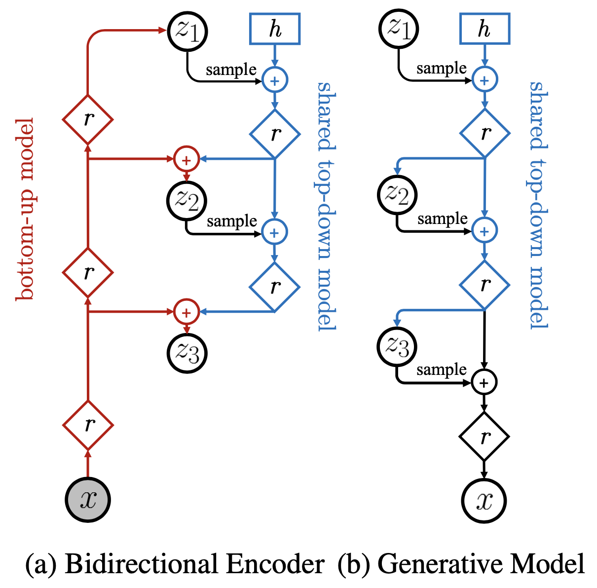
NVAE cleverly designs a multi-scale encoder and decoder, as shown above. First, the encoder goes through layers of encoding to obtain the top-level encoding vector z_1, and then gradually moves from the top down to obtain lower-level features z_2,\dots,z_L. As for the decoder, it is naturally a top-down process of utilizing z_1,z_2,\dots,z_L. Since this part shares similarities with the encoder’s process of generating z_1,z_2,\dots,z_L, NVAE directly makes the corresponding parts share parameters. This saves parameters and improves generalization through mutual constraints.
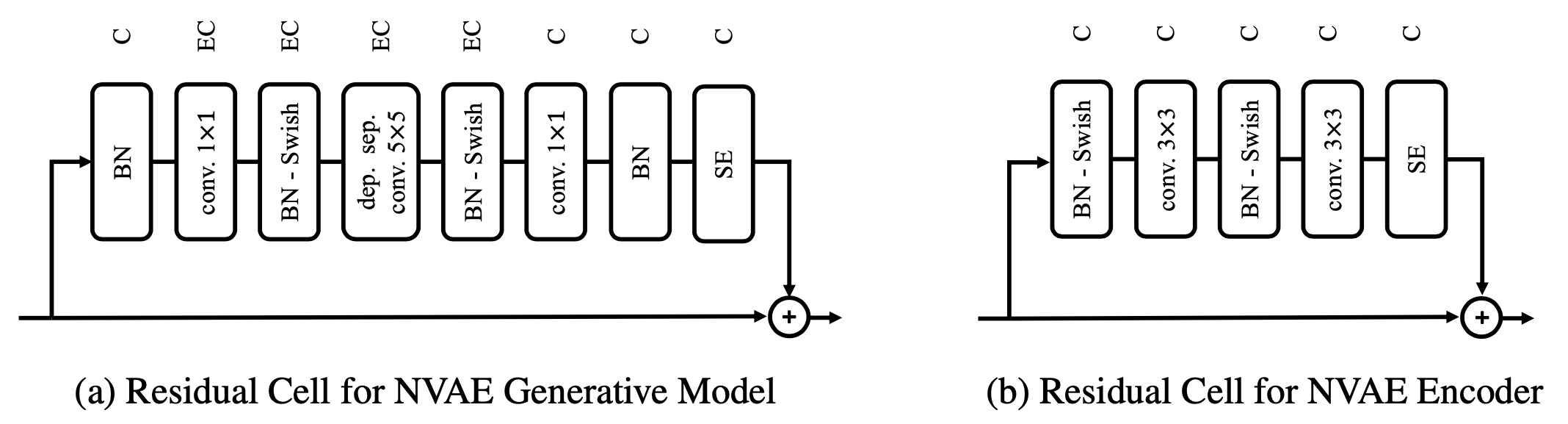
This multi-scale design is reflected in almost all current state-of-the-art generative models, such as StyleGAN, BigGAN, and VQ-VAE-2, proving its effectiveness. Furthermore, to ensure performance, NVAE carefully screened residual module designs, finally settling on the following residual block:
Other Enhancement Techniques
Besides the two obvious features above, NVAE includes many other tricks that improve performance. Here are a few.
Improvements to BN layers. Many current generative models have abandoned BN (Batch Normalization), mostly switching to IN (Instance Normalization) or WN (Weight Normalization). NVAE found through experiments that BN is actually helpful for training but harmful for prediction because the moving average mean and variance used during prediction aren’t good enough. Therefore, after training, NVAE re-estimates the mean and variance by sampling batches of the same size multiple times. Additionally, to ensure training stability, NVAE adds a regularization term to the magnitude of BN’s \gamma.
Application of Spectral Regularization. To stabilize training, NVAE adds spectral regularization to every convolutional layer (refer to my "Lipschitz Constraints in Deep Learning: Generalization and Generative Models"). Adding spectral normalization reduces the model’s Lipschitz constant, making the model’s landscape smoother and more conducive to stable training.
Flow models to enhance distributions. NVAE provides an alternative: modeling the intra-group distribution as a flow model to enhance expressiveness while maintaining parallel intra-group sampling.
Memory-saving tricks. NVAE uses mixed-precision training and promotes their own APEX library. It also enables gradient checkpointing (recomputation) in BN, which reportedly saves 18% of memory with almost no impact on speed.
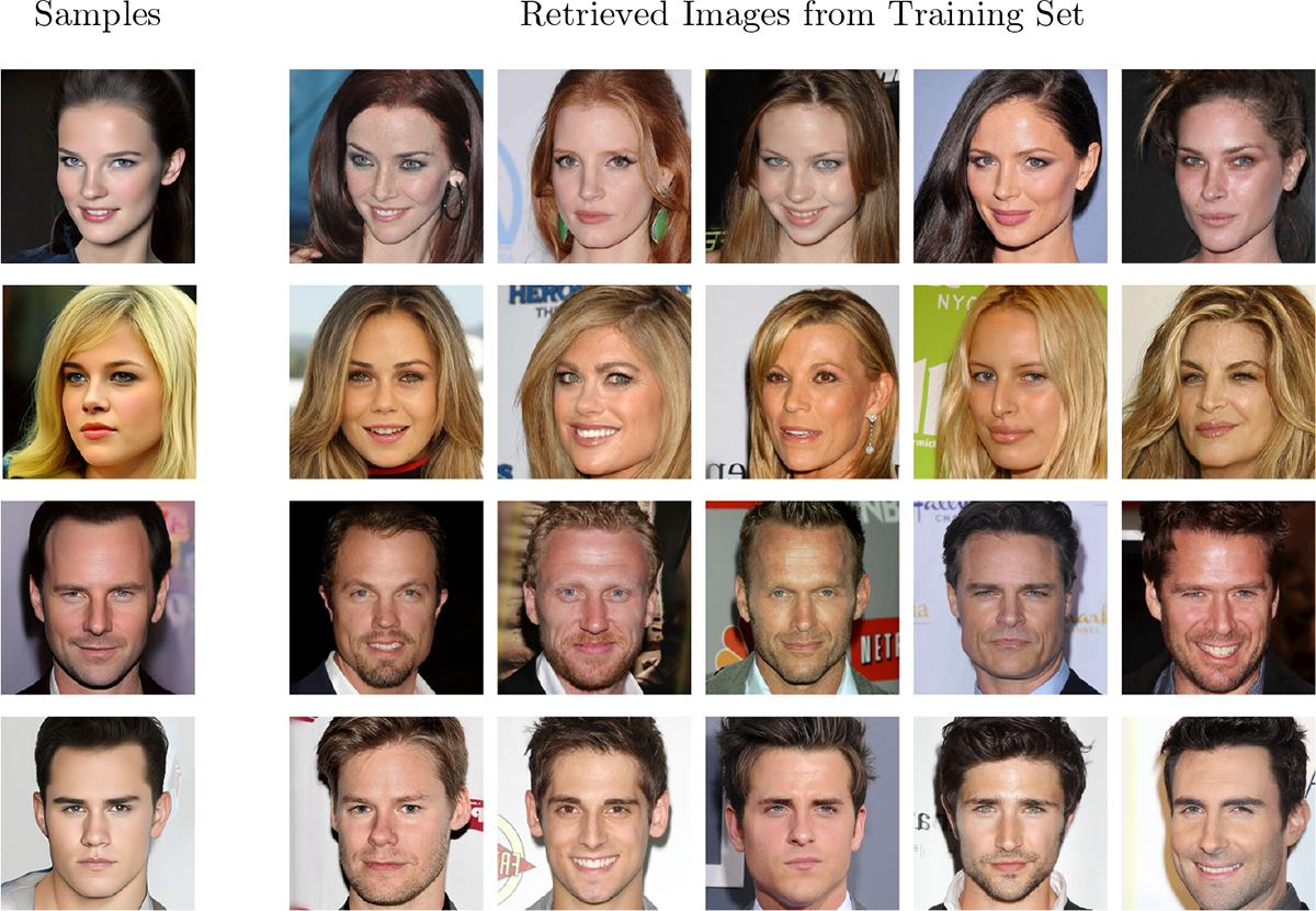
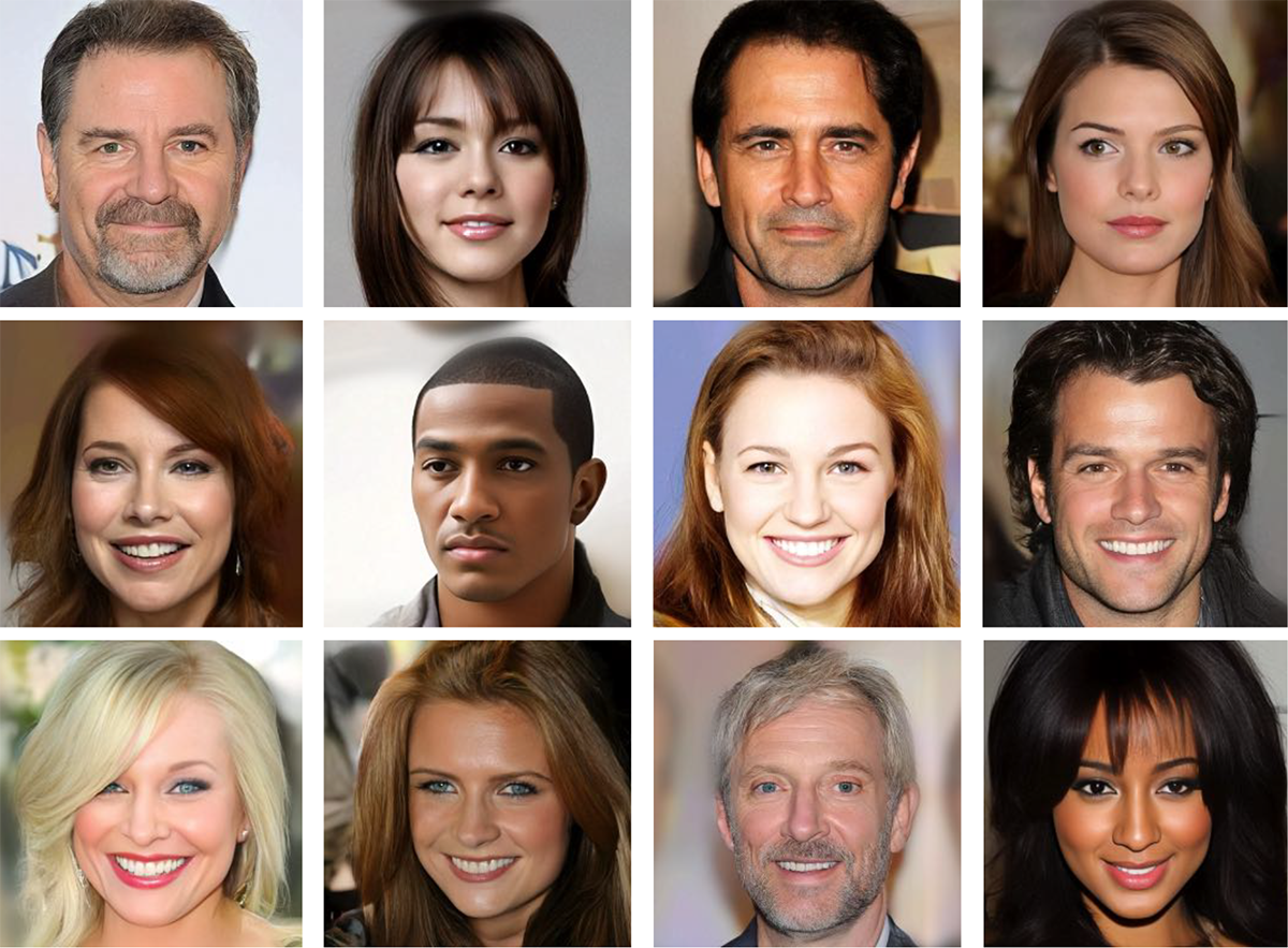
More Results
Personal Takeaways
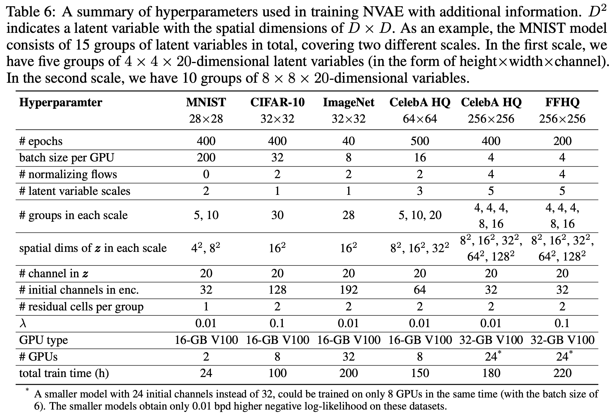
Looking at the training table below, we can see that the training cost is quite high—higher than StyleGAN at the same resolution.
For me, NVAE brings two major conceptual impacts.
First, autoregressive Gaussian models can very effectively fit complex continuous distributions. NVAE proves that even if latent variables are continuous, autoregressive Gaussians can fit well. Thus, one doesn’t necessarily have to follow the VQ-VAE discretization path.
Second, VAE latent variables can be more than one; they can be multiple and hierarchical. Looking at the table again, for the FFHQ column, regarding the latent variable z, there are 4+4+4+8+16=36 groups in total. Calculating this, to generate a 256\times 256 FFHQ image, it requires a random vector of total size: \left(4\times 8^2 + 4\times 16^2 + 4\times 32^2 + 8\times 64^2 + 16\times 128^2 \right)\times 20=6,005,760 dimensions. This is very different from traditional VAEs, which usually encode an image into a single (few-hundred-dimensional) vector.
What is Nouveau?
Finally, I curiously searched for the meaning of "Nouveau." Here is the explanation from Wikipedia:
nouveau (/nuːˈvoʊ/) is a free and open-source graphics device driver for Nvidia video cards and the Tegra family of systems-on-chips written by independent software engineers, with minor help from Nvidia employees.
The project’s goal is to create an open-source driver by reverse-engineering Nvidia’s proprietary Linux drivers. It is managed by the X.Org Foundation, hosted by freedesktop.org, and distributed as part of Mesa 3D. The project was originally based on the "nv" free and open-source driver, which only had 2D drawing capabilities, but Red Hat developer Matthew Garrett and others stated that the original code was obfuscated. nouveau is licensed under the MIT License.
The name of the project comes from the French word "nouveau", meaning "new". The name was suggested by the original author’s IRC client’s auto-replace feature, which suggested "nouveau" when he typed "nv".
Does this mean that Nouveau VAE and Nvidia VAE are essentially synonyms? It seems our initial understanding wasn’t wrong after all!
Summary
This article introduced the upgraded VAE called NVAE recently published by NVIDIA, which pushes VAE generation to a new height. As seen in the paper, NVAE raises the theoretical ceiling through autoregressive latent distributions, designs a clever encoder-decoder structure, and integrates almost all state-of-the-art techniques in current generative models, making it the strongest VAE to date.
When reposting, please include the original address of this article: https://kexue.fm/archives/7574
For more detailed reposting matters, please refer to: "Scientific Space FAQ"