Recently, I learned about a BERT model compression method called “BERT-of-Theseus,” which comes from the paper “BERT-of-Theseus: Compressing BERT by Progressive Module Replacing.” This is a model compression scheme built on the starting point of “replaceability.” Compared to conventional pruning, distillation, and other means, its entire process appears more elegant and concise. This article will provide a brief introduction to the method, present an implementation based on bert4keras, and verify its effectiveness.
Model Compression
First, let’s briefly introduce model compression. However, since I am not a specialist in model compression and have not conducted a particularly systematic survey, this introduction may appear unprofessional; I ask for the reader’s understanding.
Basic Concepts
Simply put, model compression is “simplifying a large model to obtain a small model with faster inference speed.” Generally speaking, model compression involves certain sacrifices. For instance, the most obvious is that the final evaluation metrics will decrease to some extent. After all, “better and faster” free lunches are rare, so the prerequisite for choosing model compression is being able to tolerate a certain loss in precision. Secondly, the speedup from model compression usually only manifests during the prediction stage. In other words, it typically requires a longer training time. Therefore, if your bottleneck is training time, model compression may not be suitable for you.
The reason model compression takes longer is that it requires “training a large model first, then compressing it into a small model.” Readers might wonder: why not just train a small model directly? The answer is that many current experiments have shown that training a large model first and then compressing it usually results in higher final accuracy compared to training a small model directly. That is, for the same inference speed, the model obtained through compression is superior. For related discussions, refer to the paper “Train Large, Then Compress: Rethinking Model Size for Efficient Training and Inference of Transformers,” and there is also a discussion on Zhihu: “Why compress models instead of directly training a small CNN?”
Common Methods
Common model compression techniques can be divided into two major categories: 1. Directly simplifying a large model to obtain a small model; 2. Retraining a small model with the help of a large model. The commonality between these two methods is that both require training a high-performing large model first before subsequent operations.
Representative methods of the first category are Pruning and Quantization. Pruning, as the name suggests,
attempts to delete some components of the original large model to turn
it into a small model while keeping the model’s performance within an
acceptable range. Quantization refers to not changing the original model
structure but converting the model into a different numerical format
without seriously degrading performance. Usually, we build and train
models using the float32 type; switching to
float16 can speed up inference and save memory. If it can
be further converted to 8-bit integers or even 2-bit integers
(binarization), the effect on speed and memory savings will be even more
significant.
The representative method of the second category is Distillation. The basic idea of distillation is to use the output of the large model as the label for training the small model. Taking classification as an example, while actual labels are in one-hot form, the output of the large model (such as logits) contains richer signals, allowing the small model to learn better features from them. In addition to learning the output of the large model, many times, to further improve performance, the small model is also required to learn the intermediate layer results, Attention matrices, and correlation matrices of the large model. Thus, a good distillation process usually involves multiple loss functions. How to reasonably design these losses and adjust their weights is one of the research topics in the field of distillation.
Theseus
The compression method introduced in this article is called “BERT-of-Theseus,” which belongs to the second category mentioned above. That is, it also uses a large model to train a small model, but it is designed based on the replaceability of modules.
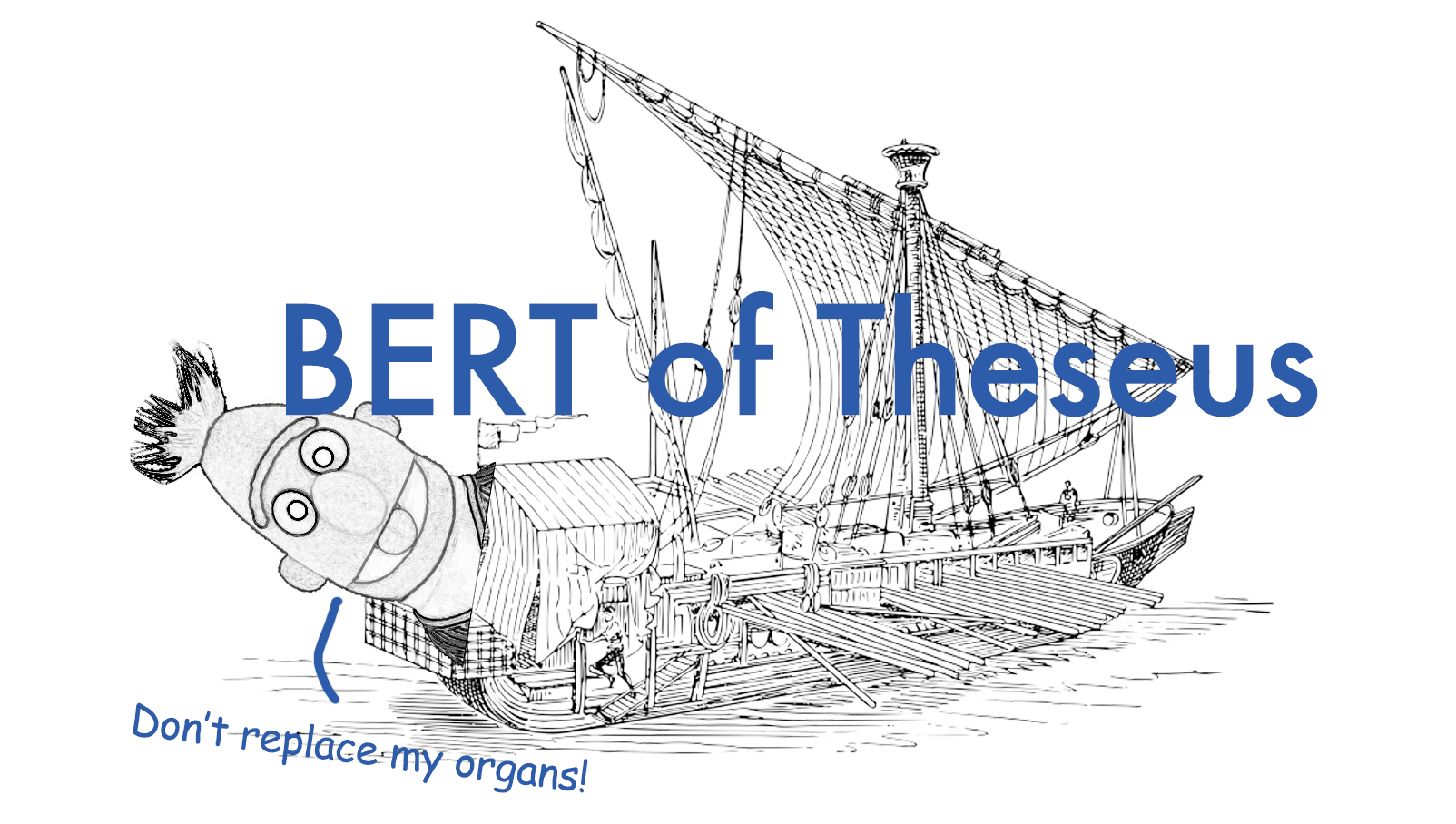
The name BERT-of-Theseus originates from the thought experiment “Ship of Theseus”: If the planks of Theseus’ ship are gradually replaced until none of the original planks remain, is it still the same ship?
Core Idea
As mentioned earlier, when using distillation for model compression, one often hopes not only that the small model’s output aligns with the large model’s output but also that the intermediate results align. What does “alignment” mean? It means replaceability! Therefore, the idea of BERT-of-Theseus is: Why bother adding various losses to achieve replaceability? Why not just replace the modules of the large model with the modules of the small model and then train them?
Consider a practical analogy:
Suppose there are two teams, A and B, each with five players. Team A is a star team with extraordinary strength; Team B is a novice team waiting to be trained. To train Team B, we select one person from Team B to replace one person in Team A, and then let this “4+1” Team A practice and compete continuously. After a period, the strength of the newly added member will improve, and this “4+1” team will possess strength close to the original Team A. Repeat this process until all members of Team B have been fully trained; eventually, the members of Team B can form a high-strength team themselves.
In contrast, if only Team B existed from the beginning and they only trained among themselves, even if their strength gradually improved, they might not reach an outstanding level without the help of the superior Team A.
Process Details
Returning to BERT compression, suppose we have a 6-layer BERT. We fine-tune it directly on a downstream task to get a well-performing model, which we call the Predecessor. Our goal is to obtain a 3-layer BERT that performs close to the Predecessor on the downstream task—at least better than directly fine-tuning the first 3 layers of BERT (otherwise, it would be a waste of effort). This small model is called the Successor. How does BERT-of-Theseus achieve this? As shown in the figures below:
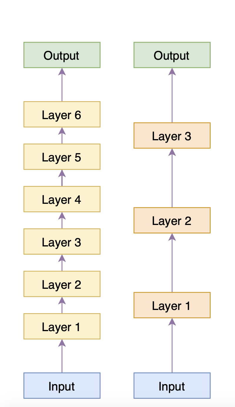
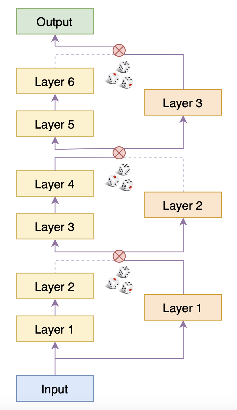
Throughout the BERT-of-Theseus process, the weights of the Predecessor are fixed. The 6-layer Predecessor is divided into 3 modules, corresponding one-to-one with the 3 layers of the Successor. During training, a Successor layer is randomly used to replace the corresponding module of the Predecessor, and then fine-tuning is performed directly using the optimization objective of the downstream task (only the Successor layers are trained). After sufficient training, the entire Successor is separated and continues to be fine-tuned on the downstream task until the validation set metrics no longer rise.
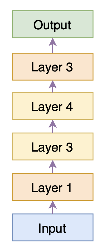
In implementation, this is actually a process similar to Dropout. Both the Predecessor and Successor models are executed, and one of the outputs of the corresponding modules is set to zero, then summed and sent to the next layer: \begin{aligned} &\varepsilon^{(l)} \sim U(\{0, 1\}) \\ &x^{(l)} = x_p^{(l)} \times \varepsilon^{(l)} + x_s^{(l)} \times \left(1 - \varepsilon^{(l)}\right) \\ &x_p^{(l+1)} = F_p^{(l+1)}\left(x^{(l)}\right) \\ &x_s^{(l+1)} = F_s^{(l+1)}\left(x^{(l)}\right) \end{aligned} Since \varepsilon is either 0 or 1 (without adjustment, a 0.5 probability for each works well), each branch effectively has only one module selected. Therefore, the diagram on the right is equivalent to the model structure. Because the zeroing is random, after enough training steps, every layer of the Successor will be well-trained.
Method Analysis
What are the advantages of BERT-of-Theseus compared to distillation? First, since this has been published, the performance should be at least comparable, so we won’t compare performance but rather the method itself. Clearly, the main characteristic of BERT-of-Theseus is: simplicity.
As mentioned before, distillation often requires matching intermediate layer outputs, which involves many training objectives: downstream task loss, intermediate layer output loss, correlation matrix loss, Attention matrix loss, etc. Thinking about balancing these losses is a headache. In contrast, BERT-of-Theseus forces the Successor to have outputs similar to the Predecessor through the replacement operation, and the final training objective is only the downstream task loss, which is remarkably concise. Furthermore, BERT-of-Theseus has a special advantage: many distillation methods must be applied to both pre-training and fine-tuning stages to achieve prominent results, whereas BERT-of-Theseus can achieve comparable results by acting directly on the fine-tuning of downstream tasks. This advantage is an experimental conclusion rather than an algorithmic one.
From a formal perspective, the random replacement idea of BERT-of-Theseus is somewhat like the data augmentation schemes SamplePairing and mixup in imaging, which both use random sampling of two objects and weighted summation to enhance the original model. It is also somewhat like the progressive training scheme of PGGAN, which achieves a transition between two models through some degree of mixing. Readers familiar with these can propose extensions or questions for BERT-of-Theseus: Does \varepsilon have to be 0 or 1? Would any random number between 0 \sim 1 work? Or, instead of being random, could \varepsilon slowly change from 1 to 0? These ideas have not yet been fully experimented with; interested readers can modify the code below to experiment themselves.
Experimental Results
The original authors have open-sourced their PyTorch implementation at JetRunner/BERT-of-Theseus. Qiu Zhenyu also shared his explanation and a TensorFlow implementation based on the original BERT at qiufengyuyi/bert-of-theseus-tf. Of course, since I decided to write this introduction, there must be a Keras implementation based on bert4keras:
This is likely the most concise and readable implementation of BERT-of-Theseus to date.
For the original paper’s results, please refer to the paper itself. I experimented on several text classification tasks, and the results were largely similar, consistent with Qiu’s experimental conclusions. The experimental results for the CLUE iflytek dataset are as follows:
| Method | Layers | Performance | |
|---|---|---|---|
| Direct Fine-tuning | 12 layers (Full) | 60.11% | |
| Direct Fine-tuning | 6 layers (First 6) | 58.99% | |
| Direct Fine-tuning | 3 layers (First 3) | 57.96% | |
| BERT-of-Theseus | 6 layers | 59.61% | |
| BERT-of-Theseus | 3 layers | 59.36% |
As can be seen, compared to directly fine-tuning the first few layers, BERT-of-Theseus indeed brings a certain performance improvement. Regarding the random zeroing scheme, besides equal probability selection of 0/1, the original paper also tried other strategies which showed slight improvements but introduced additional hyperparameters, so I did not experiment with them. Interested readers can modify and try them.
Additionally, for distillation, if the Successor has the same structure as the Predecessor (self-distillation), the final performance of the Successor is usually better than the Predecessor. Does BERT-of-Theseus have this characteristic? I experimented with this idea and found the conclusion to be negative; that is, in the case of identical models, the Successor trained by BERT-of-Theseus was not better than the Predecessor. So it seems that while BERT-of-Theseus is good, it cannot completely replace distillation.
Summary
This article introduced and experimented with a BERT model compression method called “BERT-of-Theseus.” The characteristic of this method is its clarity and simplicity, using pure replacement operations to let a small model learn the behavior of a large model, achieving state-of-the-art model compression effects with only a single loss function.
Please include the original address when reposting: https://kexue.fm/archives/7575
For more detailed reposting matters, please refer to: “Scientific Space FAQ”