Since the publication of "Attention is All You Need", Transformer models based on Multi-Head Attention have become increasingly popular. The release of the BERT model last year pushed the popularity of Transformers to a new peak. Of course, the exploration of technology is endless, and improvements have continued to emerge: some improve pre-training tasks, such as XLNet’s PLM and ALBERT’s SOP; some improve normalization, such as the shift from Post-Norm to Pre-Norm, or the removal of the beta parameter in Layer Norm in T5; some improve model structures, such as Transformer-XL; and some improve training methods, such as ALBERT’s parameter sharing.
All of the above modifications are made outside of the Attention mechanism itself, meaning they assume the rationality of Attention and do not modify it directly. In this article, we introduce two new results: they target potential modeling bottlenecks within Multi-Head Attention and propose different schemes to improve it. Both papers come from Google and are backed by extensive experiments, making their results quite persuasive.
No Matter How Small, key_size Cannot Be Too Small
The first result comes from the paper "Low-Rank Bottleneck in Multi-head Attention Models". It explicitly points out the representational bottleneck in Multi-Head Attention and proposes alleviating it by increasing the key_size.
Multi-Head Attention
First, let’s briefly review Multi-Head Attention. Readers can also refer to the previous post "A Brief Reading of ’Attention is All You Need’ (Introduction + Code)". The foundation of Multi-Head Attention is Single-Head Attention, also known as Scaled Dot-Product Attention, defined as: Attention(\boldsymbol{Q},\boldsymbol{K},\boldsymbol{V}) = \text{softmax}\left(\frac{\boldsymbol{Q}\boldsymbol{K}^{\top}}{\sqrt{d_k}}\right)\boldsymbol{V} where \boldsymbol{Q}\in\mathbb{R}^{n\times d_k}, \boldsymbol{K}\in\mathbb{R}^{m\times d_k}, \boldsymbol{V}\in\mathbb{R}^{m\times d_v}. Multi-Head Attention involves projecting \boldsymbol{Q}, \boldsymbol{K}, \boldsymbol{V} using h different sets of projection matrices, performing Single-Head Attention h times, and finally concatenating the results: \begin{aligned} &\boldsymbol{Q}^{(1)}=\boldsymbol{Q}\boldsymbol{W}_Q^{(1)},\boldsymbol{K}^{(1)}=\boldsymbol{K}\boldsymbol{W}_K^{(1)},\boldsymbol{V}^{(1)}=\boldsymbol{V}\boldsymbol{W}_V^{(1)},\boldsymbol{O}^{(1)}=Attention\left(\boldsymbol{Q}^{(1)},\boldsymbol{K}^{(1)},\boldsymbol{V}^{(1)}\right)\\ &\boldsymbol{Q}^{(2)}=\boldsymbol{Q}\boldsymbol{W}_Q^{(2)},\boldsymbol{K}^{(2)}=\boldsymbol{K}\boldsymbol{W}_K^{(2)},\boldsymbol{V}^{(2)}=\boldsymbol{V}\boldsymbol{W}_V^{(2)},\boldsymbol{O}^{(2)}=Attention\left(\boldsymbol{Q}^{(2)},\boldsymbol{K}^{(2)},\boldsymbol{V}^{(2)}\right)\\ &\qquad\qquad\qquad\qquad\vdots\\ &\boldsymbol{Q}^{(h)}=\boldsymbol{Q}\boldsymbol{W}_Q^{(h)},\boldsymbol{K}^{(h)}=\boldsymbol{K}\boldsymbol{W}_K^{(h)},\boldsymbol{V}^{(h)}=\boldsymbol{V}\boldsymbol{W}_V^{(h)},\boldsymbol{O}^{(h)}=Attention\left(\boldsymbol{Q}^{(h)},\boldsymbol{K}^{(h)},\boldsymbol{V}^{(h)}\right)\\ &\boldsymbol{O}=\left[\boldsymbol{O}^{(1)},\boldsymbol{O}^{(2)},\dots,\boldsymbol{O}^{(h)}\right] \end{aligned}
A Bottleneck in Attention
In practice, \boldsymbol{Q}, \boldsymbol{K}, \boldsymbol{V} usually have the same feature dimension d_k=d_v=d (i.e., hidden_size); for example, in BERT-Base, this is 768. The number of heads h is typically chosen as 12, 16, 24, etc. (12 for BERT-Base). Once d and h are determined, the standard choice is to set the projection matrices \boldsymbol{W}\in\mathbb{R}^{d\times (d/h)}. This means that in each Attention Head, the original d dimensions are projected to d/h dimensions before the Attention calculation. The output is also d/h dimensions, and the h results are concatenated to return to a d-dimensional output. We usually refer to d/h as the head_size.
The critical step in Attention is: \boldsymbol{P}=\text{softmax}\left(\frac{\boldsymbol{Q}\boldsymbol{K}^{\top}}{\sqrt{d_k}}\right) \label{eq:softmax} This step describes the pairwise relationship between vectors in \boldsymbol{Q} and \boldsymbol{K}. We can view \boldsymbol{P} as a binary joint distribution (technically n univariate distributions, but this detail is not crucial). If the sequence length is n, meaning each variable has n possible values, then this distribution has n^2 values.
However, after projecting \boldsymbol{Q} and \boldsymbol{K} to a lower dimension, the number of parameters for each is only n \times (d/h), totaling 2nd/h. Thus, Equation [eq:softmax] is equivalent to using 2nd/h parameters to approximate a quantity that inherently has n^2 values. Since we usually have 2nd/h \ll n^2, especially when h is large, this modeling is somewhat "over-demanding" for the model. This is the meaning of the "Low-Rank Bottleneck" mentioned in the original paper.
Why Not Try Increasing key_size?
So, what is the solution? A direct idea is to increase 2nd/h, which means either reducing the number
of heads h or increasing the
hidden_size d. However,
having more Attention Heads itself enhances the model’s representational
power, so reducing h to alleviate the
low-rank bottleneck might be counterproductive. Increasing d would naturally enhance the overall
capacity, but the model size and computational cost would explode, which
is also not an ideal choice.
Is there no other way? Yes, there is! When we project \boldsymbol{Q}, \boldsymbol{K},
\boldsymbol{V} to lower dimensions, they are usually all
projected to d/h. However, their
dimensions do not necessarily have to be equal. We only need to ensure
that the dimensions of \boldsymbol{Q}
and \boldsymbol{K} are equal (to
perform the dot product). To distinguish them, we call the dimension of
\boldsymbol{Q} and \boldsymbol{K} the key_size, while the dimension of \boldsymbol{V} is called the head_size. Changing the key_size
without changing the head_size does not affect the model’s
hidden_size.
Therefore, the solution proposed in this paper is to increase the model’s key_size. This
increases the representational power of the Attention mechanism without
changing the overall hidden_size of the model, and the
computational cost increases only slightly.
Supplementary Note:
In fact, the original paper considers increasing both
key_sizeandhead_sizesimultaneously, and then using a transformation matrix to reduce the dimension after concatenating the Multi-Head Attention outputs. However, since the concatenation and reduction step is just a linear transformation, the author believes the fundamental improvement comes from increasing thekey_size. Thus, this article emphasizes the step of increasingkey_size.Furthermore, if both
key_sizeandhead_sizeare increased, computational and memory consumption will increase significantly. If onlykey_sizeis increased, the additional resource consumption is much smaller.
Experimental Results
The idea of increasing key_size is simple and easy to
implement, but is it truly effective? Let’s look at the experimental
results from the original paper. The experiments use BERT as a baseline.
There are many charts in the paper; here is a representative one:
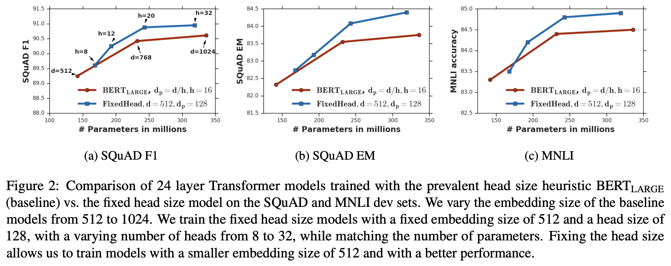
This result shows that if we fix a relatively large
key_size (e.g., 128), we can adjust the model’s
hidden_size and number of heads so that the parameter count
remains consistent with the original BERT design, yet the performance is
superior! Therefore, increasing key_size is indeed
meaningful. Even if the total parameter count is adjusted back to the
original size, it still improves the model’s performance to some extent.
This undoubtedly provides important guidance for designing new
Transformer models (especially small-scale ones).
Finally, we provide two small RoBERTa models pre-trained with
increased key_size (which we call RoBERTa^+):
No Matter What’s Missing, Talking Cannot Be Missing
The second improvement to Multi-Head Attention comes from the paper "Talking-Heads Attention". Although this paper does not explicitly mention its connection to the previous one, the author believes they are essentially solving the same problem with different approaches. It points out that in current Multi-Head Attention, the computation of each head is isolated. By linking them ("Talking"), a stronger Attention design can be achieved, hence the title "Talking-Heads Attention."
From Single Distribution to Mixture Distribution
In the previous paper, we mentioned the low-rank bottleneck: because
the key_size is too small, the representational power of
\boldsymbol{Q}^{(i)}{\boldsymbol{K}^{(i)}}^{\top}
is insufficient, so the softmax cannot properly establish a complete
binary distribution. To alleviate this, besides increasing
key_size, is there another way? Yes, such as the mixture
distribution approach used in this paper.
A mixture distribution is the superposition of multiple simple
distributions (e.g., a weighted average). It can greatly enhance the
representational power of the original distribution. A typical example
is the Gaussian Mixture Model (GMM). We know that a Gaussian
distribution is just a common simple distribution, but a Gaussian
Mixture Distribution (GMM) formed by superimposing multiple Gaussians is
a much stronger distribution. Theoretically, as long as enough Gaussians
are superimposed, a GMM can approximate any probability distribution.
This tells us that if we want to increase the representational power of
the distribution in Attention without increasing key_size,
we can consider superimposing multiple low-rank
distributions.
Where do "multiple" low-rank distributions come from? We already have Multi-Head Attention; each head provides a low-rank distribution. We can just superimpose them. This is Talking-Heads Attention. Specifically, its form is: \begin{aligned} &\hat{\boldsymbol{J}}^{(1)}=\boldsymbol{Q}^{(1)}{\boldsymbol{K}^{(1)}}^{\top},\quad\hat{\boldsymbol{J}}^{(2)}=\boldsymbol{Q}^{(2)}{\boldsymbol{K}^{(2)}}^{\top},\quad\cdots,\quad\hat{\boldsymbol{J}}^{(h)}=\boldsymbol{Q}^{(h)}{\boldsymbol{K}^{(h)}}^{\top}\\ &\begin{pmatrix}\boldsymbol{J}^{(1)} \\ \boldsymbol{J}^{(2)} \\ \vdots \\ \boldsymbol{J}^{(h)}\end{pmatrix}=\begin{pmatrix}\lambda_{11} & \lambda_{12}& \cdots & \lambda_{1h}\\ \lambda_{21} & \lambda_{22} & \cdots & \lambda_{2h}\\ \vdots & \vdots & \ddots & \vdots\\ \lambda_{h1} & \lambda_{h2} & \cdots & \lambda_{hh} \end{pmatrix}\begin{pmatrix}\hat{\boldsymbol{J}}^{(1)} \\ \hat{\boldsymbol{J}}^{(2)} \\ \vdots \\ \hat{\boldsymbol{J}}^{(h)}\end{pmatrix}\\ &\boldsymbol{P}^{(1)}=\text{softmax}\left(\boldsymbol{J}^{(1)}\right),\boldsymbol{P}^{(2)}=\text{softmax}\left(\boldsymbol{J}^{(2)}\right),\dots,\boldsymbol{P}^{(h)}=\text{softmax}\left(\boldsymbol{J}^{(h)}\right)\\ &\boldsymbol{O}^{(1)}=\boldsymbol{P}^{(1)} \boldsymbol{V}^{(1)},\quad \boldsymbol{O}^{(2)}=\boldsymbol{P}^{(2)} \boldsymbol{V}^{(2)},\quad \cdots,\quad\boldsymbol{O}^{(h)}=\boldsymbol{P}^{(h)} \boldsymbol{V}^{(h)}\\ &\boldsymbol{O}=\left[\boldsymbol{O}^{(1)},\boldsymbol{O}^{(2)},\dots,\boldsymbol{O}^{(h)}\right] \end{aligned} It looks complicated but is actually very simple: after \boldsymbol{Q}\boldsymbol{K}^{\top} and before softmax, use a parameter matrix \boldsymbol{\lambda} to superimpose the results of each \boldsymbol{Q}\boldsymbol{K}^{\top}. This links the previously isolated Attention Heads, performing a simple "Talking" step.
Two supplementary notes on the above formula:
For simplicity, the author omitted the scaling factor \sqrt{d_k}. Readers can add it back if needed.
A more general Talking-Heads Attention allows for dimensionality expansion in the \boldsymbol{J}=\boldsymbol{\lambda}\hat{\boldsymbol{J}} step, superimposing more than h mixture distributions and then reducing them with another parameter matrix. However, this is not a particularly critical improvement and is not the main focus here.
Experimental Results
Whether it is truly effective must be proven by experimental results. The experimental lineup of this paper is unprecedentedly strong, including results with BERT, ALBERT, and T5 as baselines! As is well known, BERT, ALBERT, and T5 were the state-of-the-art NLP models at various times. T5, in particular, sits at the top of the SuperGLUE leaderboard by a wide margin. Talking-Heads Attention pushes their achievements to a new height.
Again, for specific results, please refer to the paper. Here is a typical result:

This result shows that when using Talking-Head Attention, keeping
hidden_size constant, the more heads there are (and
correspondingly smaller key_size and
head_size), the better the performance. This might seem to
contradict the previous conclusion about increasing
key_size, but it actually demonstrates the significant role
of mixture distributions in improving fitting capacity. It can
superimpose simple distributions that became weaker due to smaller
key_size into a much more powerful distribution. Of course,
this doesn’t mean we should just set key_size=1, because
the computational cost at key_size=1 would be significantly
higher than the original BERT-Base. In practice, one needs to balance
performance and computation.
The table above is just the tip of the iceberg. Here is another table to show the scale of the experiments:
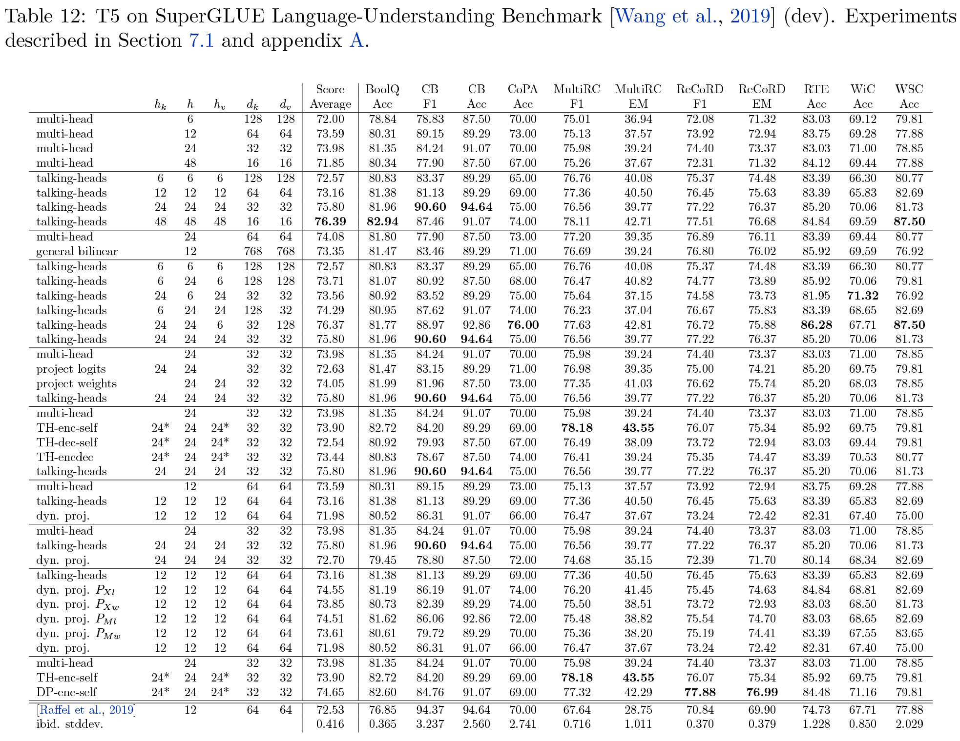
Experiments were conducted for almost every task and hyperparameter combination. Such a massive experimental lineup could basically only be produced by Google. The entire paper has a strong "T5 Style" (readers who haven’t seen the T5 paper can check "Exploring the Limits of Transfer Learning with a Unified Text-to-Text Transformer"). Unsurprisingly, one of the authors, Noam Shazeer, is also an author of T5.
The author simply wants to say that this massive experimental bombardment seems to announce to us:
Don’t doubt it; we’ve tuned all the parameters that could be tuned, and our Talking-Heads Attention is simply the best.
Interlude: A Strange Paper Style
That said, when the author first saw "Talking-Heads Attention" on arXiv, the first impression was that it might be a low-quality paper. Why? Because its style looked like this:
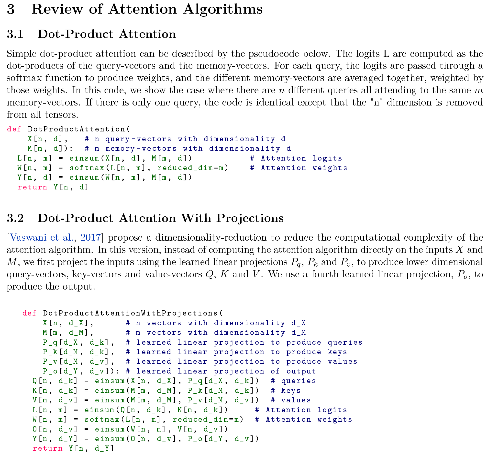
Who could imagine that such a powerful paper would contain not a single mathematical formula, replaced entirely by pseudo-code! It’s not even pseudo-code; it feels like Python code copied directly from the experiment into the main body of the paper! In the author’s memory, only low-tier papers do this. If it weren’t for a bit of patience, spotting the word "T5," and realizing the authors were all from Google, this powerful paper would have been discarded as junk.
However, such eccentricity comes at a price. Despite being effective and having a strong experimental lineup, the paper hasn’t received much of a reaction since its release over a month ago, likely due to this unconventional style.
Summary
This article introduced two subsequent works on improving Multi-Head Attention. Although the details differ, both target the "low-rank bottleneck" problem, reaching the same goal through different paths. Both works come from Google and feature rich experimental content, making the results quite persuasive. Readers working on model structure improvements may find them useful.
Reprinting should include the original address: https://kexue.fm/archives/7325
For more detailed reprinting matters, please refer to: "Scientific Space FAQ"