EAE: Autoencoder + BN + Maximum Entropy = Generative Model

Autoencoder vs. Generative Model

A standard autoencoder is a "coding-decoding" reconstruction process, as shown in the figure below:

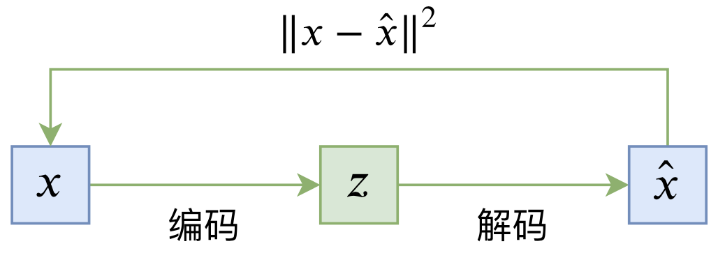
Its loss is generally: L_{AE} = \mathbb{E}_{x\sim \tilde{p}(x)}\left[\left\Vert x - \hat{x}\right\Vert^2\right] = \mathbb{E}_{x\sim \tilde{p}(x)}\left[\left\Vert x - D(E(x))\right\Vert^2\right]

Once training is complete, we can naturally obtain the encoding z=E(x) and the reconstruction \hat{x}=D(z) for any image x. When x and \hat{x} are sufficiently close, we can consider z to be an effective representation of x, as it contains sufficient information about x.

So, what is the situation with generative models? "Generation" refers to random generation, meaning it allows us to randomly construct an image. For the decoder D(z) of an autoencoder, not every z decoded results in a meaningful image. Therefore, a standard autoencoder cannot be considered a generative model. If we could know in advance the distribution of z=E(x) encoded from all x, and if this distribution were easy to sample from, then we could achieve random sampling generation.

Thus, the missing step from an autoencoder to a generative model is determining the distribution of the latent variable z, or more accurately, forcing the latent variable z to follow a simple distribution that is easy to sample from, such as a standard normal distribution. VAE achieves this by introducing a KL divergence term. How does EAE achieve it?

Normal Distribution and Maximum Entropy

We know that the Principle of Maximum Entropy is a fairly universal principle, representing our most objective cognition of unknown events. One conclusion of the Principle of Maximum Entropy is:

Among all distributions with a mean of 0 and a variance of 1, the standard normal distribution has the maximum entropy.

If readers are not yet familiar with maximum entropy, they can refer to my previous work "Too Much Entropy: From Entropy and the Maximum Entropy Principle to Maximum Entropy Models (II)". The above conclusion tells us that if we have a means to ensure the latent variable has a mean of 0 and a variance of 1, then we only need to simultaneously maximize the entropy of the latent variable to achieve the goal of "the latent variable following a standard normal distribution," i.e., \begin{aligned} &L_{EAE} = \mathbb{E}_{x\sim \tilde{p}(x)}\left[\left\Vert x - D(E(x))\right\Vert^2\right] - \lambda H(Z)\\ &\text{s.t.}\,\,\text{avg}(E(x))=0,\,\text{std}(E(x))=1 \end{aligned} where \lambda > 0 is a hyperparameter, and H(Z)=\mathbb{E}_{z\sim p(z)}[-\log p(z)] is the entropy corresponding to the latent variable z=E(x). Minimizing -\lambda H(Z) means maximizing \lambda H(Z), which is maximum entropy.

The question is: how do we ensure these two constraints? And how do we calculate the entropy of the latent variable?

Mean-Variance Constraints and BN

Let’s first solve the first problem: how to achieve—at least approximately—the constraint that "the latent variable has a mean of 0 and a variance of 1"? This is because the maximum entropy distribution is standard normal only under this constraint. The solution is the familiar Batch Normalization (BN).

During the training phase of BN, we directly subtract the mean within the batch from each variable and divide by the standard deviation within the batch. This ensures that the mean of the variables in each batch is indeed 0 and the variance is indeed 1 during training. Then, it calculates the moving average of the mean and variance of each batch and caches them for prediction during the inference phase. In short, applying BN to the latent variable allows it to (approximately) satisfy the corresponding mean and variance constraints. It should be noted that the BN layer discussed here does not include the two trainable parameters \beta and \gamma. In Keras, this means passing the parameters scale=False, center=False when initializing the BN layer.

At this point, we obtain: L_{EAE} = \mathbb{E}_{x\sim \tilde{p}(x)}\left[\left\Vert x - D(\mathcal{N}(E(x)))\right\Vert^2\right] - \lambda H(Z) \label{eq:eae} where \mathcal{N}(\cdot) represents the BN layer.

Nearest Neighbor Estimation of Entropy

Now we come to the final and most "hardcore" part of the EAE model: how to estimate the entropy H(Z). Theoretically, to calculate H(Z), we need to know p(z), but we only have samples z_1, z_2, \dots, z_n and do not know the expression for p(z). Estimating H(Z) under this premise is called non-parametric estimation.

First, the conclusion:

Nearest Neighbor Estimation of Entropy: Let z_1, z_2, \dots, z_n \in \mathbb{R}^d be n samples sampled from p(z). Let \varepsilon(i) be the distance from z_i to its nearest neighbor, i.e., \varepsilon(i) = \min_{j\neq i} \Vert z_i - z_j \Vert. Let B_d be the volume of a d-dimensional unit ball, and \gamma=0.5772\dots be the Euler-Mascheroni constant. Then: H(Z)\approx \frac{d}{n}\sum_{i=1}^n \log \varepsilon(i) + \log B_d + \log (n - 1) + \gamma \label{eq:1nn}

Setting aside the constants irrelevant to optimization, the above conclusion essentially says H(Z) \sim \sum_{i=1}^n \log \varepsilon(i). This is the term we need to add to the loss.

How is this result, which looks strange and is indeed difficult to understand, derived? In fact, it is a classic example of an important estimation method—the k-nearest neighbor method. The following derivation process is provided, referenced from the paper "A non-parametric k-nearest neighbour entropy estimator".

Let us consider a specific sample z_i. Let z_{i(k)} be its k-th nearest neighbor sample; that is, all z_j (j\neq i) are arranged in ascending order of \Vert z_j - z_i\Vert, and the k-th one is z_{i(k)}. Let \varepsilon_k(i) = \left\Vert z_i - z_{i(k)}\right\Vert. We now consider the probability distribution of \varepsilon_k(i).

Suppose \varepsilon \leq \varepsilon_k(i) \leq \varepsilon + d\varepsilon. This means that among the remaining n-1 samples, k-1 fall within the ball centered at z_i with radius \varepsilon, n-k-1 fall outside the ball centered at z_i with radius \varepsilon+d\varepsilon, and one is sandwiched between the two balls. It is not difficult to find that the probability of this occurring is: \binom{n-1}{1}\binom{n-2}{k-1}P_i(\varepsilon)^{k-1}(1 - P_i(\varepsilon + d\varepsilon))^{n-k-1}(P_i(\varepsilon + d\varepsilon) - P_i(\varepsilon)) \label{eq:dp-1} where \binom{n-1}{1} represents the number of combinations for picking 1 sample from n-1 to be between the balls, and \binom{n-2}{k-1} is the number of combinations for picking k-1 samples from the remaining n-2 to be inside the ball (the remaining n-k-1 are automatically outside). P_i(\varepsilon) is the probability of a single sample being inside the ball, i.e., P_i(\varepsilon) = \int_{\Vert z - z_i\Vert \leq \varepsilon} p(z)dz So P_i(\varepsilon)^{k-1} is the probability that the k-1 selected samples are all inside the ball, (1 - P_i(\varepsilon + d\varepsilon))^{n-k-1} is the probability that n-k-1 samples are all outside, and P_i(\varepsilon + d\varepsilon) - P_i(\varepsilon) is the probability that one sample is between the balls. Multiplying all terms gives Equation [eq:dp-1]. Expanding and keeping only the first-order terms yields the approximation: \binom{n-1}{1}\binom{n-2}{k-1}P_i(\varepsilon)^{k-1}(1 - P_i(\varepsilon))^{n-k-1}dP_i(\varepsilon) \label{eq:dp-2} Note that the above expression describes a valid probability distribution, so its integral must be 1.

Now we can make an approximate assumption. It is worth noting that this is the only assumption in the entire derivation process, and the reliability of the final result depends on how well this assumption holds: p(z_i) \approx \frac{1}{B_d \varepsilon_k(i)^d}\int_{\Vert z - z_i\Vert \leq \varepsilon} p(z)dz = \frac{P_i(\varepsilon)}{B_d \varepsilon_k(i)^d} where B_d \varepsilon_k(i)^d is the volume of the ball with radius \varepsilon_k(i). According to this approximation, we have p(z_i) B_d \varepsilon_k(i)^d \approx P_i(\varepsilon). This looks unreasonable because the left side is like a constant while the right side is a function of \varepsilon; how can they remain approximate? In fact, when n is large enough, the sampled points are dense enough, so \varepsilon will be concentrated in a relatively small range, and \varepsilon_k(i) is a sampled value of \varepsilon. Thus, we can assume \varepsilon is concentrated near \varepsilon_k(i). Although P_i(\varepsilon) varies with \varepsilon, we will integrate over \varepsilon later, so we only need the approximation of P_i(\varepsilon) to be good near \varepsilon_k(i); it doesn’t need to be a good approximation overall (i.e., when \varepsilon \gg \varepsilon_k(i), [eq:dp-2] is almost 0). Near \varepsilon_k(i), we can assume the probability change is smooth, so p(z_i) B_d \varepsilon_k(i)^d \approx P_i(\varepsilon).

Now we can write: \log p(z_i) \approx \log P_i(\varepsilon) - \log B_d - d \log \varepsilon_k(i) Multiply both sides by [eq:dp-2] and integrate over \varepsilon (the interval is [0, +\infty), or equivalently integrate over P_i in [0, 1]). Except for \log P_i(\varepsilon), the other terms are independent of \varepsilon, so they remain the same after integration, while: \begin{aligned} &\int_0^1 \binom{n-1}{1}\binom{n-2}{k-1}P_i(\varepsilon)^{k-1}(1 - P_i(\varepsilon))^{n-k-1} \log P_i(\varepsilon) d P_i(\varepsilon) \\ =&\psi(k)-\psi(n) \end{aligned} where \psi represents the digamma function. (Don’t ask me how these integrals are calculated; I don’t know, but I know Mathematica can calculate them all!)

Thus we get the approximation: \log p(z_i) \approx \psi(k)-\psi(n) - \log B_d - d \log \varepsilon_k(i) So the final approximation for entropy is: \begin{aligned} H(Z)=&\, \mathbb{E}_{z\sim p(z)}[-\log p(z)]\\ \approx&\, -\frac{1}{n}\sum_{i=1}^n \log p(z_i)\\ \approx&\, \frac{d}{n}\sum_{i=1}^n \log \varepsilon_k(i) + \log B_d + \psi(n)-\psi(k) \end{aligned} \label{eq:knn} This is a more general result than Equation [eq:1nn]. In fact, Equation [eq:1nn] is a special case of the above when k=1, because \psi(1)=-\gamma and \psi(n)= \sum_{m=1}^{n-1}\frac{1}{m}-\gamma\approx \log(n-1). These transformation formulas can be found on Wikipedia.

As mentioned at the beginning, the k-nearest neighbor method is a very useful non-parametric estimation method, and it is also related to the IMLE model I introduced previously. However, I am not very familiar with the k-nearest neighbor method myself and still need to learn more. The material I have found so far is "Lectures on the Nearest Neighbor Method". Additionally, regarding entropy estimation, one can refer to the Stanford material "Theory and Practice of Differential Entropy Estimation".

Further Thinking and Analysis

With [eq:1nn] or [eq:knn], the EAE loss described in [eq:eae] is complete, and thus the EAE model is fully introduced. The rest are experimental results, which I won’t introduce in detail; essentially, the generated images feel similar to VAE, but the metrics are better.

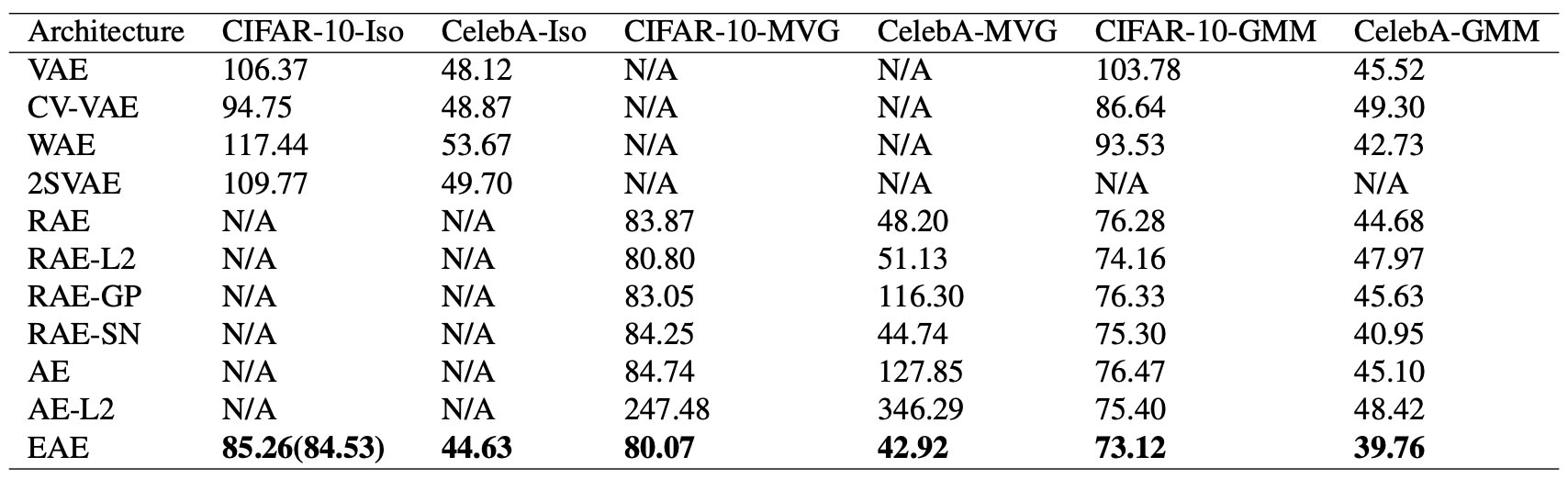
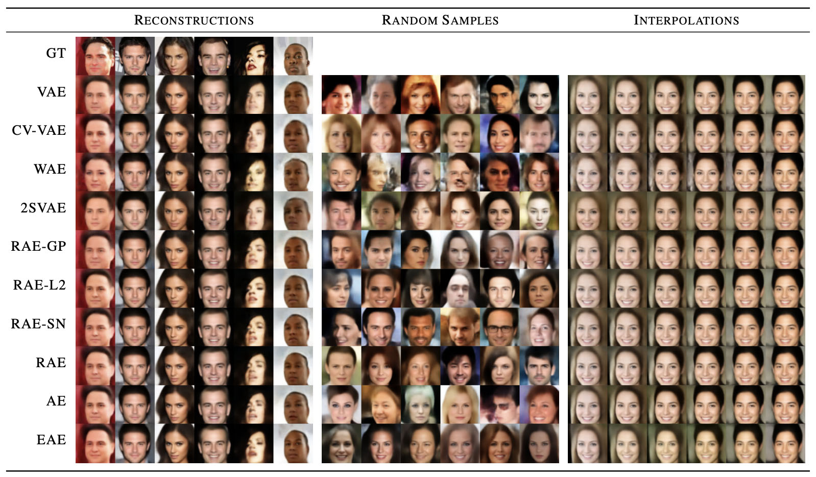
So what are the advantages of EAE compared to VAE? In VAE, a key step is reparameterization (refer to my "Variational Autoencoders (I): So That’s How It Is"). This step reduces the variance of model training (compared to REINFORCE, the variance is smaller; refer to my "Talking about Reparameterization: From Normal Distribution to Gumbel Softmax"), allowing VAE to be trained effectively. However, although reparameterization reduces variance, the variance is still not small. Simply put, the reparameterization step introduces significant noise (especially in early training), which prevents the decoder from utilizing the encoder’s information well. A typical example is the "KL vanishing" phenomenon when VAE is used in NLP.

However, EAE basically does not have this problem because EAE is essentially a standard autoencoder. The added BN does not affect the autoencoding performance, and the added entropy regularization term, in principle, only increases the diversity of the latent variables without bringing obvious difficulties to the utilization and reconstruction of encoded information. I believe this is the advantage of EAE over VAE. Of course, I have not yet conducted many experiments on EAE, and the above analysis is mostly subjective inference; readers should judge for themselves. If I have further experimental conclusions, I will continue to share them on the blog.

A Brief Summary

This article introduced a model called EAE, which mainly integrates a BN layer and maximum entropy into a standard autoencoder, giving it the capabilities of a generative model. Several experiments in the original paper show that EAE performs better than VAE, making it a model worth learning and trying. Furthermore, the key part of EAE is estimating entropy through the k-nearest neighbor method. This part is quite hardcore but actually very valuable and worth a careful read for readers interested in statistical estimation.

Please include the original address when reposting: https://kexue.fm/archives/7343

For more detailed reposting matters, please refer to: "Scientific Space FAQ"