JoSE: Joint Spherical Embedding for Word and Sentence Vectors

Optimization Objective

Conceptually, this paper is essentially consistent with Doc2Vec: to train sentence vectors, a sentence is represented by an ID and treated as a word that co-occurs with all words within that sentence. Finally, a Skip-Gram model is trained using negative sampling. The difference from Doc2Vec is that JoSE normalizes the lengths of all vectors (i.e., it only considers vectors on a unit sphere), and the training objective uses a hinge loss instead of cross-entropy:

\max(0, m - \cos(\boldsymbol{u}, \boldsymbol{v}) - \cos(\boldsymbol{u}, \boldsymbol{d}) + \cos(\boldsymbol{u}', \boldsymbol{v}) + \cos(\boldsymbol{u}', \boldsymbol{d})) \label{eq:loss}

Where \boldsymbol{u} is the word vector of the "center word," \boldsymbol{v} is the word vector of the "context word" (they come from two separate word vector spaces), \boldsymbol{d} is the sentence vector of the current sentence, and \boldsymbol{u}' is the word vector of a "center word" obtained through negative sampling. The constant m > 0 is a margin. Readers who have worked on similarity models should easily understand the meaning of this optimization objective: it aims to ensure that the "word-word-sentence" score \cos(\boldsymbol{u}, \boldsymbol{v}) + \cos(\boldsymbol{u}, \boldsymbol{d}) within a sentence is higher than the "word-random word-sentence" score \cos(\boldsymbol{u}', \boldsymbol{v}) + \cos(\boldsymbol{u}', \boldsymbol{d}), but not excessively so—only higher by the margin m.

Assuming \boldsymbol{u}, \boldsymbol{v}, \boldsymbol{d} are already normalized (and treated as column vectors), the objective [eq:loss] becomes:

\max(0, m - \boldsymbol{v}^{\top}\boldsymbol{u} - \boldsymbol{d}^{\top}\boldsymbol{u} + \boldsymbol{v}^{\top} \boldsymbol{u}' + \boldsymbol{d}^{\top} \boldsymbol{u}') \label{eq:loss2}

Gradient Descent

The objective [eq:loss] or [eq:loss2] is not particularly novel. Like most word vector objectives, it uses the inner product to measure word correlation. Since the vectors here are normalized, the inner product is simply the cosine similarity. As for whether hinge loss or cross-entropy is superior, I suspect there isn’t a significant difference.

In fact, I find the paper’s subsequent geometric analysis of the gradient more interesting. I will repeat the derivation process in my own words here. Let \boldsymbol{x} be one of the vectors among all \boldsymbol{u}, \boldsymbol{v}, \boldsymbol{d}. Suppose we fix all other vectors and optimize only \boldsymbol{x}. Let the total loss be f(\boldsymbol{x}). This optimization process can be described in two ways:

\mathop{\text{argmin}}_{\boldsymbol{x},\,\Vert\boldsymbol{x}\Vert=1} f(\boldsymbol{x}) \quad \text{or} \quad \mathop{\text{argmin}}_{\boldsymbol{\theta}} f\left(\frac{\boldsymbol{\theta}}{\Vert \boldsymbol{\theta}\Vert}\right)

In other words, we can understand this as a minimization problem of f(\boldsymbol{x}) subject to the constraint \Vert \boldsymbol{x}\Vert=1, or we can transform it into an unconstrained minimization problem of f(\boldsymbol{\theta}/\Vert\boldsymbol{\theta}\Vert) by setting \boldsymbol{x}=\boldsymbol{\theta}/\Vert\boldsymbol{\theta}\Vert. Since constrained optimization is often less intuitive, we follow the latter approach.

Unlike complex models, word vectors are relatively simple, so it is best to manually derive the gradient form and write a corresponding function for gradient descent rather than relying on automatic differentiation tools. For f(\boldsymbol{\theta}/\Vert\boldsymbol{\theta}\Vert), it is not difficult to derive:

\nabla_{\boldsymbol{\theta}}\,f\left(\frac{\boldsymbol{\theta}}{\Vert \boldsymbol{\theta}\Vert}\right) = \frac{1}{\Vert\boldsymbol{\theta}\Vert}\left(\boldsymbol{I} - \boldsymbol{x}\boldsymbol{x}^{\top}\right)\nabla_{\boldsymbol{x}}\,f\left(\boldsymbol{x}\right)

where \boldsymbol{x}=\boldsymbol{\theta}/\Vert\boldsymbol{\theta}\Vert has been substituted back into parts of the expression. Based on this result, the iteration formula for gradient descent is:

\boldsymbol{\theta}_{t+1} = \boldsymbol{\theta}_{t} - \eta_t\left(\boldsymbol{I} - \boldsymbol{x}_t\boldsymbol{x}_t^{\top}\right)\nabla_{\boldsymbol{x}_t}\,f\left(\boldsymbol{x}_t\right)

where \eta_t is the learning rate at the current moment, and the factor 1/\Vert\boldsymbol{\theta}\Vert is integrated into the learning rate since it is just a scalar. We can then write:

\begin{aligned} \boldsymbol{x}_{t+1} = \frac{\boldsymbol{\theta}_{t+1}}{\Vert \boldsymbol{\theta}_{t+1}\Vert} &= \frac{\boldsymbol{\theta}_{t} - \eta_t\left(\boldsymbol{I} - \boldsymbol{x}_t\boldsymbol{x}_t^{\top}\right)\nabla_{\boldsymbol{x}_t}\,f\left(\boldsymbol{x}_t\right)}{\left\Vert \boldsymbol{\theta}_{t} - \eta_t\left(\boldsymbol{I} - \boldsymbol{x}_t\boldsymbol{x}_t^{\top}\right)\nabla_{\boldsymbol{x}_t}\,f\left(\boldsymbol{x}_t\right)\right\Vert}\\ &= \frac{\boldsymbol{x}_{t} - \eta_t/\Vert\boldsymbol{\theta}\Vert\times\left(\boldsymbol{I} - \boldsymbol{x}_t\boldsymbol{x}_t^{\top}\right)\nabla_{\boldsymbol{x}_t}\,f\left(\boldsymbol{x}_t\right)}{\left\Vert \boldsymbol{x}_{t} - \eta_t/\Vert\boldsymbol{\theta}\Vert\times\left(\boldsymbol{I} - \boldsymbol{x}_t\boldsymbol{x}_t^{\top}\right)\nabla_{\boldsymbol{x}_t}\,f\left(\boldsymbol{x}_t\right)\right\Vert} \end{aligned}

Integrating 1/\Vert\boldsymbol{\theta}\Vert into the learning rate again, we obtain the update formula involving only \boldsymbol{x}_t:

\boldsymbol{x}_{t+1} = \frac{\boldsymbol{x}_{t} - \eta_t\left(\boldsymbol{I} - \boldsymbol{x}_t\boldsymbol{x}_t^{\top}\right)\nabla_{\boldsymbol{x}_t}\,f\left(\boldsymbol{x}_t\right)}{\left\Vert \boldsymbol{x}_{t} - \eta_t\left(\boldsymbol{I} - \boldsymbol{x}_t\boldsymbol{x}_t^{\top}\right)\nabla_{\boldsymbol{x}_t}\,f\left(\boldsymbol{x}_t\right)\right\Vert}

Update Magnitude Correction

Up to this point, the derivation has been quite standard. What follows is the interesting part. First, observe that:

\begin{aligned} \boldsymbol{g} &= \left(\boldsymbol{I} - \boldsymbol{x}_t\boldsymbol{x}_t^{\top}\right)\nabla_{\boldsymbol{x}_t}\,f\left(\boldsymbol{x}_t\right)\\ &= \nabla_{\boldsymbol{x}_t}\,f\left(\boldsymbol{x}_t\right) - \boldsymbol{x}_t\boldsymbol{x}_t^{\top}\nabla_{\boldsymbol{x}_t}\,f\left(\boldsymbol{x}_t\right)\\ &= \nabla_{\boldsymbol{x}_t}\,f\left(\boldsymbol{x}_t\right) - \boldsymbol{x}_t\Vert \nabla_{\boldsymbol{x}_t}\,f\left(\boldsymbol{x}_t\right)\Vert \cos\left(\boldsymbol{x}_t,\nabla_{\boldsymbol{x}_t}\,f\left(\boldsymbol{x}_t\right)\right) \end{aligned}

It can be seen that \boldsymbol{x}_t\boldsymbol{x}_t^{\top}\nabla_{\boldsymbol{x}_t}\,f\left(\boldsymbol{x}_t\right) is actually the projection of the vector \nabla_{\boldsymbol{x}_t}\,f\left(\boldsymbol{x}_t\right) onto the direction of \boldsymbol{x}_t. Thus, \boldsymbol{g} is a vector perpendicular to \boldsymbol{x}_t, as shown in the figure below:

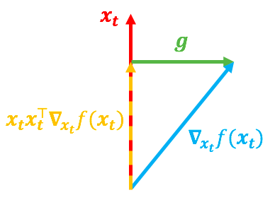
In the figure above, the red vector represents \boldsymbol{x}_t and the blue vector represents \nabla_{\boldsymbol{x}_t}\,f\left(\boldsymbol{x}_t\right). If there were no constraint \Vert \boldsymbol{x}\Vert=1, the update would be directly determined by \nabla_{\boldsymbol{x}_t}\,f\left(\boldsymbol{x}_t\right). However, because of the constraint, the update is determined by \boldsymbol{g}=\left(\boldsymbol{I} - \boldsymbol{x}_t\boldsymbol{x}_t^{\top}\right)\nabla_{\boldsymbol{x}_t}\,f\left(\boldsymbol{x}_t\right). Nevertheless, two different \nabla_{\boldsymbol{x}_t}\,f\left(\boldsymbol{x}_t\right) can lead to the same \boldsymbol{g}:

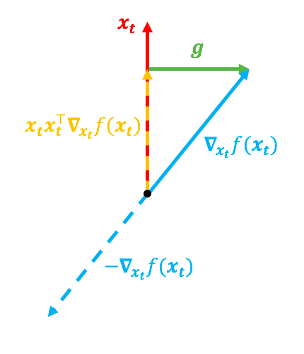
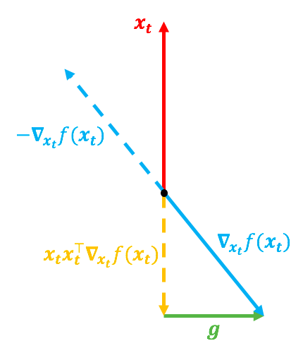
In the first case, the direction of \nabla_{\boldsymbol{x}_t}\,f\left(\boldsymbol{x}_t\right) is very close to \boldsymbol{x}_t; in the second case, it is the opposite. But their \boldsymbol{g} is identical. As mentioned, without constraints, -\nabla_{\boldsymbol{x}_t}\,f\left(\boldsymbol{x}_t\right) would be the reasonable update direction. With constraints, while -\nabla_{\boldsymbol{x}_t}\,f\left(\boldsymbol{x}_t\right) cannot point to the most reasonable gradient direction, intuitively, it should still be related to the update magnitude.

In the first case, -\nabla_{\boldsymbol{x}_t}\,f\left(\boldsymbol{x}_t\right) is far from the direction of \boldsymbol{x}_t, implying the update magnitude should be larger. In the second case, -\nabla_{\boldsymbol{x}_t}\,f\left(\boldsymbol{x}_t\right) is more aligned with \boldsymbol{x}_t. Since we only care about the direction of \boldsymbol{x}_{t+1} and not its magnitude, the update magnitude should logically be smaller in this case.

Therefore, even if \boldsymbol{g} is the same in both cases, we still need to distinguish between them. A natural idea is: since the consistency of the directions of -\nabla_{\boldsymbol{x}_t}\,f\left(\boldsymbol{x}_t\right) and \boldsymbol{x}_t affects the update magnitude, we might use:

1-\cos(-\nabla_{\boldsymbol{x}_t}\,f\left(\boldsymbol{x}_t\right),\boldsymbol{x}_t)=1+\frac{\boldsymbol{x}_t^{\top}\nabla_{\boldsymbol{x}_t}\,f\left(\boldsymbol{x}_t\right)}{\left\Vert \nabla_{\boldsymbol{x}_t}\,f\left(\boldsymbol{x}_t\right)\right\Vert}

to adjust the update magnitude. This adjustment factor satisfies the property that "the more consistent the directions, the smaller the factor." This natural idea leads to the final update formula:

\boldsymbol{x}_{t+1} = \frac{\boldsymbol{x}_{t} - \eta_t\left(1+\frac{\boldsymbol{x}_t^{\top}\nabla_{\boldsymbol{x}_t}\,f\left(\boldsymbol{x}_t\right)}{\left\Vert \nabla_{\boldsymbol{x}_t}\,f\left(\boldsymbol{x}_t\right)\right\Vert}\right)\left(\boldsymbol{I} - \boldsymbol{x}_t\boldsymbol{x}_t^{\top}\right)\nabla_{\boldsymbol{x}_t}\,f\left(\boldsymbol{x}_t\right)}{\left\Vert \boldsymbol{x}_{t} - \eta_t\left(1+\frac{\boldsymbol{x}_t^{\top}\nabla_{\boldsymbol{x}_t}\,f\left(\boldsymbol{x}_t\right)}{\left\Vert \nabla_{\boldsymbol{x}_t}\,f\left(\boldsymbol{x}_t\right)\right\Vert}\right)\left(\boldsymbol{I} - \boldsymbol{x}_t\boldsymbol{x}_t^{\top}\right)\nabla_{\boldsymbol{x}_t}\,f\left(\boldsymbol{x}_t\right)\right\Vert}

Unnecessary Complexity

Having discussed the interesting parts, let’s move to the less interesting ones. Readers with a slightly deeper understanding of NLP (those who have read the mathematical principles of Word2Vec and derived gradients for standard models) might feel that the content of the first two sections is not particularly profound. The geometric interpretation and learning rate adjustment in the third section are somewhat novel but follow a logical path. However, if you read the original paper, the experience might be quite different. The authors use language like "probability distributions" and "optimization on Riemannian manifolds," making content that should be relatively easy to understand feel obscure and unnecessarily complicated.

First, one point I find difficult to understand is that the authors start with an unreasonable assumption (continuizing word vectors) and spend considerable space arguing that p(v|u)\sim e^{\cos(\boldsymbol{v},\boldsymbol{u})} and p(u|d)\sim e^{\cos(\boldsymbol{u},\boldsymbol{d})} correspond to the Von Mises–Fisher distribution. And then? Nothing. All subsequent content has almost nothing to do with this Von Mises–Fisher distribution, so I don’t understand the purpose of including that part.

Next, in the optimization section, the authors state that the minimization of f(\boldsymbol{x}) under the constraint \Vert\boldsymbol{x}\Vert=1 cannot be solved with gradient descent, so "Riemannian Gradient Descent" must be used. Then they begin to "show off": discussing Riemannian manifolds, providing general exponential maps, and then Riemannian gradients. After all these high-end operations, they ultimately settle on a solution everyone can understand: \boldsymbol{x}=\boldsymbol{\theta}/\Vert\boldsymbol{\theta}\Vert. At this point, I was quite "impressed." While the author’s logic and derivations are correct, why go through all that to give the reader the simple result of \boldsymbol{x}=\boldsymbol{\theta}/\Vert\boldsymbol{\theta}\Vert? Why not just discuss the optimization of f(\boldsymbol{x}=\boldsymbol{\theta}/\Vert\boldsymbol{\theta}\Vert) from the start? Is it necessary to confuse ordinary readers with Riemannian manifolds?

Furthermore, the part I found interesting—the geometric explanation of the update magnitude and the resulting adjustment factor—was also described quite vaguely by the authors. In short, I believe many parts of the paper’s theoretical derivation are filled with unnecessary technical jargon, which needlessly increases the difficulty for ordinary readers.

Finally, I want to emphasize that I never oppose "multiple solutions to one problem," nor do I oppose deepening or abstracting simple content. "Deepening" and "abstraction" can indeed lead to a more comprehensive understanding or reveal connections between different branches. However, such "deepening" and "abstraction" should be built upon a simple solution that most people can understand, rather than intentionally discarding the simple solution for the sake of complexity.

Experimental Results

Critiques aside, JoSE performs very well in the experimental section. First, an efficient C implementation of JoSE is provided:

Github: https://github.com/yumeng5/Spherical-Text-Embedding

I tried it out, and the training is indeed very fast. The trained word/sentence vectors can be loaded using gensim’s KeyedVectors. I also looked at the source code; it is concise, clear, and easy to modify.

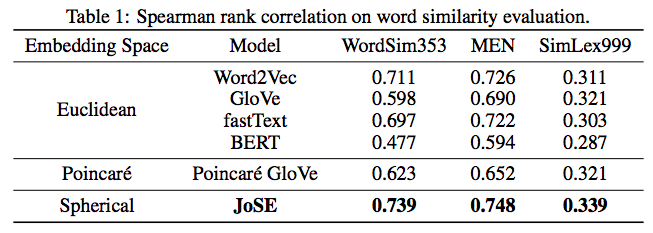
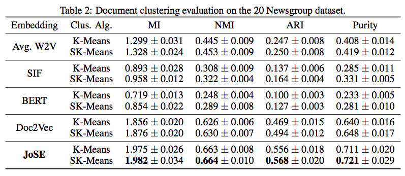
As for the experimental results, JoSE is quite leading in the word/sentence vector evaluations provided in the paper:

Conclusion

This article shared JoSE, a text vector model published at NeurIPS 2019, focusing on the parts I found inspiring and providing my own derivation process. JoSE can be considered a natural variant of Doc2Vec with subtle adjustments and the author’s own insights into optimization methods. Aside from some parts that seem unnecessarily complicated, it remains a noteworthy piece of work.

Original URL: https://kexue.fm/archives/7063