Yesterday, there was a discussion in our group about some counter-intuitive phenomena regarding n-dimensional vectors. One topic was: “In general n-dimensional space, two random vectors are almost always orthogonal.” This significantly differs from our intuition in two-dimensional or three-dimensional space. To understand this conclusion theoretically, we can consider the distribution of the angle \theta between two random vectors and calculate its mean and variance.
Probability Density
First, let us derive the probability density function (PDF) of \theta. Actually, there is not much derivation needed; it is a direct consequence of n-dimensional hyperspherical coordinates.
To find the distribution of the angle between two random vectors, it is clear that due to isotropy, we only need to consider unit vectors. Furthermore, because of isotropy, we can fix one vector and consider the other vector as varying randomly. Without loss of generality, consider the random vector as: \boldsymbol{x}=(x_1,x_2,\dots,x_n) And the fixed vector as: \boldsymbol{y}=(1,0,\dots,0)
Transform \boldsymbol{x} into hyperspherical coordinates (for knowledge about n-dimensional spheres, refer to Wikipedia): \left\{\begin{aligned} x_{1}&=\cos(\varphi_{1})\\ x_{2}&=\sin(\varphi_{1})\cos(\varphi_{2})\\ x_{3}&=\sin(\varphi_{1})\sin(\varphi_{2})\cos(\varphi_{3})\\ &\,\,\vdots \\ x_{n-1}&=\sin(\varphi_{1})\cdots \sin(\varphi_{n-2})\cos(\varphi_{n-1})\\ x_{n}&=\sin(\varphi_{1})\cdots \sin(\varphi_{n-2})\sin(\varphi_{n-1}) \end{aligned}\right. Where \varphi_{n-1}\in [0, 2\pi) and the remaining \varphi ranges are [0, \pi]. At this point, the angle between \boldsymbol{x} and \boldsymbol{y} is: \arccos \langle \boldsymbol{x},\boldsymbol{y}\rangle = \arccos \cos(\varphi_{1}) = \varphi_{1} That is to say, the angle between the two is exactly \varphi_1. Then, the probability that the angle between \boldsymbol{x} and \boldsymbol{y} does not exceed \theta is: P_n(\varphi_1\leq\theta) = \frac{\text{Integral on the } n\text{-dimensional hypersphere where } \varphi_1 \text{ does not exceed } \theta}{\text{Total integral on the } n\text{-dimensional hypersphere}} The differential volume element on the n-dimensional hypersphere is \sin^{n-2}(\varphi_{1})\sin^{n-3}(\varphi_{2})\cdots \sin(\varphi_{n-2})\,d\varphi_{1}\,d\varphi_{2}\cdots d\varphi_{n-1} (which can be found on Wikipedia), so: \begin{aligned} P_n(\varphi_1\leq\theta) &= \frac{\int_0^{2\pi}\cdots\int_0^{\pi}\int_0^{\theta}\sin^{n-2}(\varphi_{1})\sin^{n-3}(\varphi_{2})\cdots \sin(\varphi_{n-2})\,d\varphi_{1}\,d\varphi_{2}\cdots d\varphi_{n-1}}{\int_0^{2\pi}\cdots\int_0^{\pi}\int_0^{\pi}\sin^{n-2}(\varphi_{1})\sin^{n-3}(\varphi_{2})\cdots \sin(\varphi_{n-2})\,d\varphi_{1}\,d\varphi_{2}\cdots d\varphi_{n-1}}\\ &=\frac{(n-1)\text{-dimensional unit hypersphere surface area} \times \int_0^{\theta}\sin^{n-2}\varphi_{1} d\varphi_1}{n\text{-dimensional unit hypersphere surface area}}\\ &=\frac{\Gamma\left(\frac{n}{2}\right)}{\Gamma\left(\frac{n-1}{2}\right)\sqrt{\pi}} \int_0^{\theta}\sin^{n-2}\varphi_1 d\varphi_1 \end{aligned} This indicates that the probability density function of \theta is: p_n(\theta) = \frac{\Gamma\left(\frac{n}{2}\right)}{\Gamma\left(\frac{n-1}{2}\right)\sqrt{\pi}}\sin^{n-2} \theta \label{eq:theta} Sometimes we are interested in the distribution of \eta=\cos\theta. In this case, we need to perform a change of variables for the probability density: \begin{aligned} p_n(\eta)&=\frac{\Gamma\left(\frac{n}{2}\right)}{\Gamma\left(\frac{n-1}{2}\right)\sqrt{\pi}}\sin^{n-2} (\arccos\eta)\left|\frac{d\theta}{d\eta}\right|\\ &=\frac{\Gamma\left(\frac{n}{2}\right)}{\Gamma\left(\frac{n-1}{2}\right)\sqrt{\pi}}(1-\eta^2)^{(n-3)/2}\\ \end{aligned}\label{eq:cos}
Distribution Characteristics
From equations [eq:theta] and [eq:cos], we can see that when n=2, the distribution of the angle \theta is a uniform distribution, and when n=3, the distribution of the cosine of the angle \cos\theta is a uniform distribution. These two results show that in the two-dimensional and three-dimensional spaces we perceive, the distribution of angles is relatively uniform. But what about when n is large? For example, n=20 or 50?
From the form p_n(\theta)\sim\sin^{n-2}\theta, we can find that when n\geq 3, the maximum probability occurs at \theta=\frac{\pi}{2} (i.e., 90 degrees). Additionally, \sin^{n-2}\theta is symmetric about \theta=\frac{\pi}{2}, so its mean is also \frac{\pi}{2}. However, this does not fully describe the distribution; we also need to consider the variance: Var_n(\theta) = \frac{\Gamma\left(\frac{n}{2}\right)}{\Gamma\left(\frac{n-1}{2}\right)\sqrt{\pi}}\int_0^{\pi}\left(\theta-\frac{\pi}{2}\right)^2\sin^{n-2} \theta d\theta This integral has an analytical solution, but the form is quite cumbersome (if you are interested, you can calculate it yourself using Mathematica). Let’s look at some numerical solutions:
| n | Variance |
|---|---|
| 3 | 0.467401 |
| 10 | 0.110661 |
| 20 | 0.0525832 |
| 50 | 0.0204053 |
| 100 | 0.0101007 |
| 200 | 0.00502508 |
| 1000 | 0.001001 |
As can be seen, as n increases, the variance becomes smaller and smaller. This means that in high-dimensional space, the angle between any two vectors is almost always concentrated around \frac{\pi}{2}. In other words, in high-dimensional space, any two vectors are almost always orthogonal.
Of course, this can also be seen from the plot:
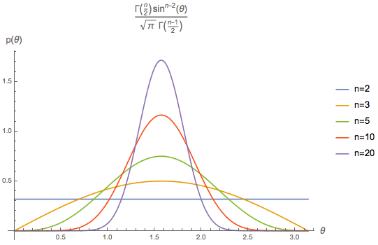
For readers who want an approximate analytical solution, consider using Laplace’s method to approximate p_n(\theta) with a Gaussian distribution: expand \ln \sin^{n-2}\theta at \theta=\frac{\pi}{2}: \ln \sin^{n-2}\theta=\frac{2-n}{2}\left(\theta - \frac{\pi}{2}\right)^2 + \mathcal{O}\left(\left(\theta - \frac{\pi}{2}\right)^4\right) That is: \sin^{n-2}\theta\approx \exp\left[-\frac{n-2}{2}\left(\theta - \frac{\pi}{2}\right)^2\right] From this approximate form, we can approximately consider that \theta follows a normal distribution with a mean of \frac{\pi}{2} and a variance of \frac{1}{n-2}. That is, when n is large, the variance is approximately \frac{1}{n-2}, which also shows that the larger n is, the smaller the variance.
Summary
This article derives the distribution of angles in high-dimensional space, recorded here for future reference and for the benefit of interested readers.
Original address: https://kexue.fm/archives/7076
For more details on reprinting, please refer to: Scientific Space FAQ