What BERT is probably doesn’t need much introduction from me. Although I am not particularly fond of BERT, I must admit that it has indeed caused a massive stir in the NLP community. Currently, whether in Chinese or English, popular science explanations and interpretations of BERT are everywhere, arguably surpassing the momentum of Word2Vec when it first arrived. Interestingly, BERT was created by Google, and Word2Vec was also created by Google. No matter which one you use, you are following in the footsteps of the giants at Google.
Shortly after BERT was released, some readers suggested I write an interpretation, but I ultimately didn’t. Firstly, there are already many interpretations of BERT. Secondly, BERT is essentially a large-scale corpus pre-trained model based on Attention; it isn’t a major technical innovation in itself. Since I have already written an interpretation of Google’s Attention, I didn’t feel particularly motivated to write another.
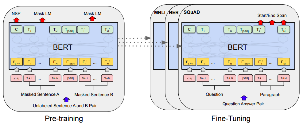
Overall, I personally had little interest in BERT until late last month when I first tried it during an information extraction competition. I later realized that even if I wasn’t interested, I still needed to learn it—after all, whether to use it is one thing, but knowing how to use it is another. Furthermore, there don’t seem to be many articles introducing how to use (fine-tune) BERT within Keras, so I decided to share my experience.
When BERT Meets Keras
Fortunately, some developers have already encapsulated a Keras version of BERT, which can directly call the pre-trained weights released officially. For readers who already have some foundation in Keras, this might be the simplest way to invoke BERT. The phrase "standing on the shoulders of giants" perfectly describes the feeling of Keras enthusiasts right now.
keras-bert
In my opinion, the best encapsulation of BERT for Keras currently is:
keras-bert: https://github.com/CyberZHG/keras-bert
This article is based on this library.
As a side note, besides keras-bert, the developer
CyberZHG has also encapsulated many other valuable Keras modules, such
as keras-gpt-2 (allowing you to use the GPT-2 model like
BERT), keras-lr-multiplier (for setting learning rates
layer by layer), keras-ordered-neurons (the ON-LSTM introduced recently),
and more. A summary can be found here. It seems he is a
die-hard Keras fan. Respect to the
developer.
In fact, with keras-bert and a bit of basic Keras
knowledge—and given that the demos provided by keras-bert
are quite comprehensive—calling and fine-tuning BERT has become a task
with very little technical barrier. Therefore, I will simply provide a
few Chinese examples to help readers get started with the basic usage of
keras-bert.
Tokenizer
Before diving into the examples, it is necessary to discuss the
Tokenizer. We import BERT’s Tokenizer and
reconstruct it:
from keras_bert import load_trained_model_from_checkpoint, Tokenizer
import codecs

config_path = '../bert/chinese_L-12_H-768_A-12/bert_config.json'
checkpoint_path = '../bert/chinese_L-12_H-768_A-12/bert_model.ckpt'
dict_path = '../bert/chinese_L-12_H-768_A-12/vocab.txt'

token_dict = {}
with codecs.open(dict_path, 'r', 'utf8') as reader:
    for line in reader:
        token = line.strip()
        token_dict[token] = len(token_dict)

class OurTokenizer(Tokenizer):
    def _tokenize(self, text):
        R = []
        for c in text:
            if c in self._token_dict:
                R.append(c)
            elif self._is_space(c):
                R.append('[unused1]') # Represent spaces with untrained [unused1]
            else:
                R.append('[UNK]') # Remaining characters are [UNK]
        return R

tokenizer = OurTokenizer(token_dict)
tokenizer.tokenize(u'The weather is nice today')
# Output is ['[CLS]', u'The', ..., '[SEP]'] (Note: Example shown for Chinese characters in original)
Here is a brief explanation of the Tokenizer output. By
default, the [CLS] and [SEP] tokens are added
to the beginning and end of the tokenized sentence, respectively. The
output vector corresponding to the [CLS] position is
designed to represent the entire sentence vector, while
[SEP] is the separator between sentences. The rest are
single-character outputs (for Chinese).
Originally, Tokenizer has its own _tokenize
method. I rewrote it here to ensure that the tokenized result has the
same length as the original string (plus 2 for the markers). The
built-in _tokenize automatically removes spaces and merges
some characters, causing the tokenized list
length to differ from the original string length, which makes
sequence labeling tasks very troublesome. To avoid this, it’s better to
rewrite it. We use [unused1] to represent space-like
characters, and other characters not in the list are represented by
[UNK]. The [unused*] tokens are untrained
(randomly initialized) and reserved by BERT for incrementally adding
vocabulary, so we can use them to represent any new characters.
Three Examples
Here are three examples using keras-bert: Text Classification, Relation Extraction, and
Subject Extraction. All
are done by fine-tuning the officially released pre-trained weights.
Official BERT Github: https://github.com/google-research/bert
Official Chinese Pre-trained Weights: chinese_L-12_H-768_A-12.zip
Examples Github: https://github.com/bojone/bert_in_keras/
According to the official description, these weights were trained using the Chinese Wikipedia as the corpus.
(Updated June 20, 2019: The Joint Laboratory of HIT and iFLYTEK
released a new version of weights that can also be loaded with
keras_bert. Details can be found here.)
Text Classification
As the first example, we will perform a basic text classification task. Once you are familiar with this, other tasks will become quite simple. We will use the sentiment classification task discussed many times before, using the labeled data compiled previously.
Let’s look at the model part (full code available here):
# Note: Although seq_len=None can be set, ensure sequence length does not exceed 512
bert_model = load_trained_model_from_checkpoint(config_path, checkpoint_path, seq_len=None)

for l in bert_model.layers:
    l.trainable = True

x1_in = Input(shape=(None,))
x2_in = Input(shape=(None,))

x = bert_model([x1_in, x2_in])
x = Lambda(lambda x: x[:, 0])(x) # Extract the vector corresponding to [CLS] for classification
p = Dense(1, activation='sigmoid')(x)

model = Model([x1_in, x2_in], p)
model.compile(
    loss='binary_crossentropy',
    optimizer=Adam(1e-5), # Use a sufficiently small learning rate
    metrics=['accuracy']
)
model.summary()
And that’s it for sentiment classification using BERT in Keras!
Does it feel like the model code ended before you even got started?
Calling BERT in Keras is just that short. In fact, the only line that
truly "calls" BERT is load_trained_model_from_checkpoint;
the rest are standard Keras operations (thanks again to CyberZHG). So,
if you have already started with Keras, calling BERT is effortless.
With such a simple call, what accuracy can be achieved? After 5 epochs of fine-tuning, the best accuracy on the validation set is 95.5%+! Previously, in "Text Sentiment Classification (III): To Segment or Not to Segment", we struggled to reach around 90% accuracy; with BERT, a few lines of code improved the accuracy by over 5 percentage points! No wonder BERT has caused such a craze in the NLP world...
Based on my personal experience, let me answer two questions readers might be concerned about.
The first question is likely: "How much VRAM is enough?" In fact, there is no standard answer. VRAM usage depends on three factors: sentence length, batch size, and model complexity. For the sentiment analysis example above, it can run on a GTX 1060 with 6GB VRAM by simply adjusting the batch size to 24. So, if your VRAM is insufficient, try reducing the
maxlenandbatch size. Of course, if your task is too complex, even the smallestmaxlenandbatch sizemight lead to OOM (Out of Memory), in which case you’ll need to upgrade your GPU.The second question is: "Are there any principles for what layers to add after BERT?" The answer is: Use as few layers as possible to complete your task. For example, the sentiment analysis above is just a binary classification task, so you just take the first vector and add a
Dense(1). Don’t think about adding multiple Dense layers, and definitely don’t think about adding an LSTM followed by Dense. If you are doing sequence labeling (like NER), just addDense+CRF. In short, add as little extra as possible. First, BERT itself is complex enough and has the capacity to handle many tasks; second, the layers you add are randomly initialized, and adding too many can cause violent perturbations to BERT’s pre-trained weights, potentially reducing effectiveness or even preventing convergence.
Relation Extraction
If the reader already has a foundation in Keras, then after the first example, you should have completely mastered fine-tuning BERT because it is truly too simple to require much explanation. Therefore, the following two examples mainly provide reference patterns to help you understand how to "use as few layers as possible."
In the second example, we introduce a minimalist relation extraction model based on BERT. The labeling principle is the same as introduced in "A Lightweight Information Extraction Model Based on DGCNN and Probabilistic Graphs", but thanks to BERT’s powerful encoding capabilities, the code we write can be greatly simplified. In the reference implementation I provided, the model part is as follows (full model here):
t = bert_model([t1, t2])
ps1 = Dense(1, activation='sigmoid')(t)
ps2 = Dense(1, activation='sigmoid')(t)

subject_model = Model([t1_in, t2_in], [ps1, ps2]) # Model to predict subject

k1v = Lambda(seq_gather)([t, k1])
k2v = Lambda(seq_gather)([t, k2])
kv = Average()([k1v, k2v])
t = Add()([t, kv])
po1 = Dense(num_classes, activation='sigmoid')(t)
po2 = Dense(num_classes, activation='sigmoid')(t)

object_model = Model([t1_in, t2_in, k1_in, k2_in], [po1, po2]) # Input text and subject, predict object and relation

train_model = Model([t1_in, t2_in, s1_in, s2_in, k1_in, k2_in, o1_in, o2_in],
                    [ps1, ps2, po1, po2])
If you have read the article on the DGCNN-based model and understand the architecture without BERT, you will realize how concise and clear the above implementation is.
As you can see, we introduced BERT as the encoder to get the encoded
sequence t, then directly connected two
Dense(1) layers to complete the subject labeling model.
Next, we extract the encoding vectors corresponding to the start and end
of the passed s, add them to the encoding vector sequence
t, and then connect two
Dense(num_classes) layers to complete the object labeling
model (simultaneously labeling the relation).
With such a simple design, what is the final F1 score? The answer:
The offline dev set reached nearly 82%, and an
online submission I made once resulted in 85%+ (both single
models)! In contrast, the model in the DGCNN article required
CNNs, global features, passing s into an LSTM for encoding,
and relative position vectors. Various "brainstormed" modules were fused
together, and the single model was only slightly better (about 82.5%).
Keep in mind that I wrote this BERT-based model in just one hour, while
I spent nearly two months tuning the DGCNN model with all its tricks!
The power of BERT is evident.
(Note: Fine-tuning this model preferably requires more than 8GB of VRAM. Additionally, because I only encountered BERT a few days before the competition ended and wrote this model then, I didn’t spend much time tuning it, so the final submission did not include BERT.)
A noticeable difference between this relation extraction example and the previous sentiment analysis example is the change in learning rate.
In the sentiment analysis example, we used a constant learning rate (10^{-5}) for a few epochs, and the results were quite good. In this relation extraction example, the learning rate for the first epoch gradually increases from 0 to 5 \times 10^{-5} (this is called warmup), and the second epoch decreases from 5 \times 10^{-5} back to 10^{-5}. Overall, it increases then decreases. BERT itself was trained with a similar learning rate curve; this training method is more stable, less likely to collapse, and generally yields better results.
Event Subject Extraction
The final example comes from the CCKS 2019 Event Subject Extraction in the Financial Domain. This competition is still ongoing, but I no longer have the motivation or interest to continue, so I am releasing my current model (accuracy 89%+) for reference. I wish the remaining contestants the best of luck.
Briefly, the data for this competition looks like this:
Input: "Company A’s product contained additives, and its subsidiaries B and C were investigated", "Product issues"
Output: "Company A"
In other words, this is a dual-input, single-output model. The input is a query and an event type, and the output is an entity (there is one and only one, and it is a fragment of the query). This task can be seen as a simplified version of SQuAD 1.0. Given the output characteristics, a pointer structure is better (two softmax layers predicting the start and end). The remaining question is: how to handle dual inputs?
While the previous two examples varied in complexity, they were both single-input. What about dual inputs? Of course, there are only a limited number of entity types, so direct Embedding would work. However, I used a solution that better demonstrates BERT’s "brute force" strength: directly concatenate the two inputs into one sentence using a separator, turning it into a single-input problem! For example, the sample above is processed as:
Input: "___Product issues___Company A’s product contained additives, and its subsidiaries B and C were investigated"
Output: "Company A"
Then it becomes a standard single-input extraction problem. Speaking of which, there isn’t much to say about the code for this model; it’s just a few lines (full code here):
x = bert_model([x1, x2])
ps1 = Dense(1, use_bias=False)(x)
ps1 = Lambda(lambda x: x[0][..., 0] - (1 - x[1][..., 0]) * 1e10)([ps1, x_mask])
ps2 = Dense(1, use_bias=False)(x)
ps2 = Lambda(lambda x: x[0][..., 0] - (1 - x[1][..., 0]) * 1e10)([ps2, x_mask])

model = Model([x1_in, x2_in], [ps1, ps2])
With some decoding tricks and model ensemble, the submission reached 89%+. Looking at the current leaderboard, the best result is just over 90%, so I suspect everyone is doing something similar... (The results of this code fluctuate during repeated experiments; you may need to run it several times to get the optimal result.)
This example primarily teaches us that when implementing your own tasks with BERT, it is best to organize them into a single-input format. This is simpler and more efficient.
For instance, in a sentence similarity model where you input two sentences and output a similarity score, there are two approaches. The first is to pass each sentence through the same BERT separately and use their respective
[CLS]features for classification. The second is to concatenate the two sentences with a marker into one sentence, pass it through BERT, and classify the output features. The latter is clearly faster and allows for more comprehensive interaction between features.
Summary
This article introduced the basic method of calling BERT in Keras, primarily providing three reference examples to help everyone gradually become familiar with the steps and principles of fine-tuning BERT. Much of this is based on my own experience; if there are any inaccuracies, I hope readers will correct me.
In fact, with the keras-bert library implemented by
CyberZHG, using BERT in Keras is a piece of cake. After half a day of
tinkering, you’ll get the hang of it. Finally, I wish everyone a
pleasant experience using it!
When reposting, please include the original address: https://kexue.fm/archives/6736
For more details on reposting, please refer to: "Scientific Space FAQ"