A Discussion on Reparameterization: From Normal Distribution to Gumbel Softmax

Form

From Equation [eq:lianxu], we know that L_{\theta} in the continuous case actually corresponds to an integral. Therefore, to explicitly write L_{\theta}, there are two paths: The most direct way is to accurately complete the integral [eq:lianxu] to obtain an explicit expression, but this is usually impossible; thus, the only way is to transform it into the sampling form [eq:base] and attempt to preserve the gradient of \theta during the sampling process.

Reparameterization is such a technique. It assumes that sampling from the distribution p_{\theta}(z) can be decomposed into two steps: (1) Sample an \varepsilon from a parameter-less distribution q(\varepsilon); (2) Generate z through a transformation z=g_{\theta}(\varepsilon). Then, Equation [eq:base] becomes: L_{\theta}=\mathbb{E}_{\varepsilon\sim q(\varepsilon)}[f(g_{\theta}(\varepsilon))] \label{eq:reparam} At this point, the sampled distribution has no parameters; they have all been transferred inside f. Therefore, we can sample several points and write them down like a standard loss function.

Example

The simplest example is the normal distribution: for a normal distribution, reparameterization changes "sampling a z from \mathcal{N}\left(z;\mu_{\theta},\sigma_{\theta}^2\right)" into "sampling an \varepsilon from \mathcal{N}\left(\varepsilon;0, 1\right), and then calculating \varepsilon\times \sigma_{\theta} + \mu_{\theta}." Thus: \mathbb{E}_{z\sim \mathcal{N}\left(z;\mu_{\theta},\sigma_{\theta}^2\right)}\big[f(z)\big] = \mathbb{E}_{\varepsilon\sim \mathcal{N}\left(\varepsilon;0, 1\right)}\big[f(\varepsilon\times \sigma_{\theta} + \mu_{\theta})\big]

How to understand why direct sampling has no gradient while reparameterization does? It’s quite simple. For example, if I say sample a number from \mathcal{N}\left(z;\mu_{\theta},\sigma_{\theta}^2\right) and you tell me you sampled 5, I cannot see any relationship between 5 and \theta (the gradient can only be 0). However, if we first sample a number like 0.2 from \mathcal{N}\left(\varepsilon;0, 1\right) and then calculate 0.2 \sigma_{\theta} + \mu_{\theta}, then I know the relationship between the sampled result and \theta (an effective gradient can be calculated).

Summary

Let’s reorganize the previous content. Overall, reparameterization in the continuous case is relatively simple: we need to handle L_{\theta} as in Equation [eq:lianxu]. Since we cannot explicitly write out the exact integral, we need to convert it into sampling. To obtain effective gradients during sampling, we need reparameterization.

From a mathematical perspective, reparameterization is an integral transformation. That is, the original integral was with respect to z, and through the transformation z=g_{\theta}(\varepsilon), a new integral form is obtained.

Analysis

When readers see the summation in [eq:lisan], their first reaction might be: "Summation? Then just sum it, it’s not like it’s impossible."

Indeed, that was my first reaction as well. Unlike the continuous case in [eq:lianxu], which would require completing an integral (which can be seen as a sum of infinite points) if tackled directly, the discrete case in [eq:lisan] is just a sum of finite terms. Theoretically, one could indeed complete the summation and then perform gradient descent.

However, what if k is extremely large? For example, if y is a 100-dimensional vector where each element is either 0 or 1 (binary variables), the total number of different y values is 2^{100}. Summing over 2^{100} terms is computationally unacceptable. Another typical example is the decoder side of seq2seq (which must be faced if doing text GANs), where the total number of categories is |V|^l, where |V| is the vocabulary size and l is the sentence length. In such cases, completing the exact summation is unfeasible.

Form

Therefore, we still need to return to sampling. If we can sample a few points to get an effective estimate of [eq:lisan] without losing gradient information, that would be ideal. To this end, we first introduce Gumbel Max, which provides a method for sampling from a categorical distribution.

Suppose the probability of each category is p_1, p_2, \dots, p_k. The following process provides a scheme for sampling categories according to these probabilities, known as Gumbel Max: \mathop{\text{argmax}}_i \Big(\log p_i - \log(-\log \varepsilon_i)\Big)_{i=1}^k,\quad \varepsilon_i\sim U[0, 1] In other words, first calculate the logarithm of each probability \log p_i, then sample k random numbers \varepsilon_1, \dots, \varepsilon_k from a uniform distribution U[0, 1], add -\log(-\log \varepsilon_i) to \log p_i, and finally extract the category corresponding to the maximum value.

We will prove later that this process is exactly equivalent to sampling a category according to probabilities p_1, p_2, \dots, p_k. In other words, in Gumbel Max, the probability of outputting i is exactly p_i. Since the randomness has now been transferred to U[0, 1], and U[0, 1] does not contain unknown parameters, Gumbel Max is a reparameterization process for discrete distributions.

However, we want reparameterization not to lose gradient information, but Gumbel Max cannot achieve this because \mathop{\text{argmax}} is non-differentiable. Therefore, further approximation is needed. First, note that in neural networks, the basic method for handling discrete inputs is to convert them into one-hot form (the essence of the Embedding layer is also a one-hot fully connected layer; see "What’s Really Going On with Word Vectors and Embeddings?"). Thus, \mathop{\text{argmax}} is actually \text{onehot}(\mathop{\text{argmax}}). Then, we seek a smooth approximation of \text{onehot}(\mathop{\text{argmax}}), which is softmax (see "A Discussion on Function Smoothing: Differentiable Approximation of Non-differentiable Functions").

From this, we obtain the smooth approximation version of Gumbel Max—Gumbel Softmax: \text{softmax} \Big(\big(\log p_i - \log(-\log \varepsilon_i)\big)\big/\tau\Big)_{i=1}^k,\quad \varepsilon_i\sim U[0, 1] where the parameter \tau > 0 is called the annealing parameter (temperature). The smaller it is, the closer the output is to the one-hot form (but simultaneously, the gradient vanishing problem becomes more severe). A small tip: if p_i is the output of a softmax, as in Equation [eq:softmax], there is no need to calculate p_i and then take the log; simply replace \log p_i with o_i: \text{softmax} \Big(\big(o_i - \log(-\log \varepsilon_i)\big)\big/\tau\Big)_{i=1}^k,\quad \varepsilon_i\sim U[0, 1]

Proof of Gumbel Max:

The form of Gumbel Max looks a bit complicated, far less simple than the reparameterization of a normal distribution. But in fact, as long as you have the courage to look at it, even the proof is not difficult. We want to prove that the probability of Gumbel Max outputting i is p_i. Without loss of generality, we prove the probability of outputting 1 is p_1.

Note that outputting 1 means \log p_1 - \log(-\log \varepsilon_1) is the largest, which implies: \begin{aligned} &\log p_1 - \log(-\log \varepsilon_1) > \log p_2 - \log(-\log \varepsilon_2) \\ &\log p_1 - \log(-\log \varepsilon_1) > \log p_3 - \log(-\log \varepsilon_3) \\ &\qquad \vdots\\ &\log p_1 - \log(-\log \varepsilon_1) > \log p_k - \log(-\log \varepsilon_k) \end{aligned}

Note that each inequality is independent. That is, the relationship between \log p_1 - \log(-\log \varepsilon_1) and \log p_2 - \log(-\log \varepsilon_2) does not affect its relationship with \log p_3 - \log(-\log \varepsilon_3). Thus, we only need to analyze the probability of each inequality individually. Without loss of generality, we analyze the first inequality, which simplifies to: \varepsilon_2 < \varepsilon_1^{p_2 / p_1} \leq 1 Since \varepsilon_2 \sim U[0, 1], the probability that \varepsilon_2 < \varepsilon_1^{p_2 / p_1} is \varepsilon_1^{p_2 / p_1}. This is the probability that the first inequality holds given a fixed \varepsilon_1. Then, the probability that all inequalities hold simultaneously is: \varepsilon_1^{p_2 / p_1}\varepsilon_1^{p_3 / p_1}\dots \varepsilon_1^{p_k / p_1}=\varepsilon_1^{(p_2 + p_3 + \dots + p_k) / p_1}=\varepsilon_1^{(1/p_1)-1} Then, averaging over all \varepsilon_1: \int_0^1 \varepsilon_1^{(1/p_1)-1}d\varepsilon_1 = p_1 This is the probability of category 1 appearing, which is p_1. Thus, we have completed the proof of the Gumbel Max sampling process.

Example

As in the continuous case, Gumbel Softmax is used in scenarios where one needs to calculate \mathbb{E}_{y\sim p_{\theta}(y)}[f(y)] and cannot directly complete the summation over y. In such cases, we calculate p_{\theta}(y) (or o_i), choose a \tau > 0, use Gumbel Softmax to calculate a random vector \tilde{y}, and substitute it to get f(\tilde{y}). This is a good approximation of \mathbb{E}_{y\sim p_{\theta}(y)}[f(y)] and preserves gradient information.

Note that Gumbel Softmax is not an equivalent form of categorical sampling; Gumbel Max is. Gumbel Max can be seen as the limit of Gumbel Softmax as \tau \to 0. Therefore, when applying Gumbel Softmax, one can initially choose a larger \tau (e.g., 1) and then slowly anneal it to a number close to 0 (e.g., 0.01) to obtain better results.

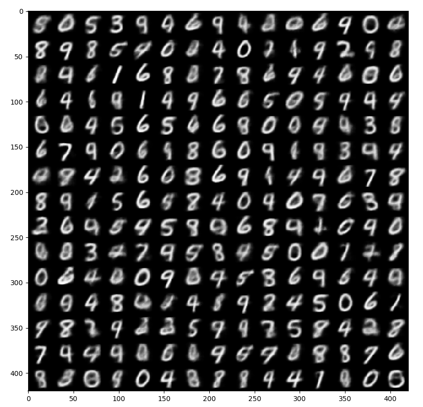
Below is an example of a discrete latent variable VAE I implemented:
https://github.com/bojone/vae/blob/master/vae_keras_cnn_gs.py

Result image:

Origins

Gumbel Max has been around for a long time, but the first paper to propose and apply Gumbel Softmax was "Categorical Reparameterization with Gumbel-Softmax". This paper mainly explored variational inference problems where some latent variables are discrete, such as semi-supervised learning based on VAE (the method is somewhat similar to "Variational Autoencoders (IV): A One-Step Clustering Scheme"). Subsequently, in the article "GANs for Sequences of Discrete Elements with the Gumbel-softmax Distribution", Gumbel Softmax was first used for discrete sequence generation, though not yet for text generation, but for simpler artificial character sequences.

Later, SeqGAN was proposed. Since then, text GAN models have mostly appeared in combination with reinforcement learning. Pure deep learning and gradient descent methods based on Gumbel Softmax remained relatively quiet until the appearance of RelGAN. RelGAN is a model proposed at ICLR 2019. It introduced a new generator and discriminator structure, allowing text GANs trained directly with Gumbel Softmax to significantly outperform previous text GAN models. We will discuss RelGAN further when the opportunity arises.

Summary

This section mainly introduced Gumbel Softmax, which is a reparameterization trick for losses of the form [eq:base] in discrete cases.

Theoretically, the discrete case of [eq:base] is just a finite summation and does not necessarily require reparameterization. However, in reality, "finite" can be a very large number, making traversal summation difficult. Thus, it still needs to be converted into a sampling form, requiring reparameterization tricks. This is Gumbel Softmax, derived from the smoothing of Gumbel Max.

In addition to the above perspective, there is an auxiliary view: Gumbel Softmax gradually approaches one-hot through \tau \to 0 annealing. Compared to annealing with the original Softmax, the difference is that the original Softmax annealing can only yield a one-hot vector where the maximum position is 1, while Gumbel Softmax has a probability of yielding a one-hot vector at non-maximum positions, increasing randomness and making sampling-based training more thorough.

SF Estimator

Previously, we discussed continuous and discrete reparameterization at the "loss level," meaning we found ways to define the loss explicitly and left the rest to the framework for automatic differentiation and optimization. In fact, even if we cannot explicitly write the loss function, it does not prevent us from taking its derivative, and naturally, it does not prevent us from using gradient descent. For example: \begin{aligned} \frac{\partial}{\partial\theta}\int p_{\theta}(z) f(z)dz &= \int f(z) \frac{\partial}{\partial\theta} p_{\theta}(z) dz\\ &= \int p_{\theta}(z)\times\frac{f(z)}{p_{\theta}(z)}\frac{\partial}{\partial\theta} p_{\theta}(z) dz\\ &= \mathbb{E}_{z\sim p_{\theta}(z)}\left[\frac{f(z)}{p_{\theta}(z)}\frac{\partial}{\partial\theta} p_{\theta}(z)\right]\\ &= \mathbb{E}_{z\sim p_{\theta}(z)}\Big[f(z)\frac{\partial}{\partial\theta} \log p_{\theta}(z)\Big] \end{aligned} \label{eq:sf} Now we have an estimation formula for the gradient, called the "SF estimator," full name Score Function Estimator. This is the most primitive estimate of the original loss function. In reinforcement learning, where z represents the policy, the above formula is a basic policy gradient, so it is sometimes directly called REINFORCE. Note that re-deriving the loss function for the discrete case yields the same result. That is, the above result is universal and does not distinguish whether z is a continuous or discrete variable. Now we can directly sample several points from p_{\theta}(z) to estimate the value of Equation [eq:sf]; there is no need to worry about whether there is a gradient, because Equation [eq:sf] itself is the gradient.

Gradient Variance

It looks beautiful—an estimation formula applicable to both continuous and discrete variables. So why do we still need reparameterization?

The main reason is: the variance of the SF estimator is too large. Equation [eq:sf] is the expectation of the function f(z) \frac{\partial}{\partial\theta} \log p_{\theta}(z) under the distribution p_{\theta}(z). We need to sample a few points to calculate it (ideally, we hope to sample only one point). In other words, we want to use the following approximation: \mathbb{E}_{z\sim p_{\theta}(z)}\Big[f(z) \frac{\partial}{\partial\theta} \log p_{\theta}(z)\Big]\approx f(\tilde{z}) \frac{\partial}{\partial\theta} \log p_{\theta}(\tilde{z}),\quad \tilde{z}\sim p_{\theta}(z) Then the problem arises: the variance of such a gradient estimate is very large.

What does it mean for the variance to be large? What is the impact? For a simple example, suppose \alpha = \text{avg}([4, 5, 6]) = \text{avg}([0, 5, 10]). That is, our target \alpha is the average of three numbers. These three numbers are either 4, 5, 6 or 0, 5, 10. In the case of exact estimation, the two are equivalent. But what if we can only randomly pick one number from each set? In the first set, we might pick 4, which is fine, as it’s only slightly different from the accurate value 5. But in the second set, we might pick 0, which is quite far from the accurate value 5. That is, in the case of picking one randomly, the fluctuation (variance) of the second set’s estimate is too large. Similarly, the gradient variance estimated by SF is like this, which leads to considerable instability when optimizing with gradient descent, making it very easy to collapse.

Variance Reduction

Formally, Equation [eq:sf] is very elegant; the form itself is not complex, it is universal for discrete and continuous variables, and it has no special requirements for f (conversely, reparameterization requires f to be differentiable, but in scenarios like reinforcement learning, f(z) corresponds to a reward function, which is hard to make smooth and differentiable). Therefore, many papers explore variance reduction techniques based on Equation [eq:sf]. The paper "Categorical Reparameterization with Gumbel-Softmax" lists some, and there have been new developments in recent years. In short, search for keywords like gradient estimator and REINFORCE, and you will find many articles.

Reparameterization is another variance reduction technique. To see this, let’s write the gradient expression for Equation [eq:reparam] after reparameterization: \begin{aligned} \frac{\partial}{\partial\theta}\mathbb{E}_{\varepsilon\sim q(\varepsilon)}[f(g_{\theta}(\varepsilon))] &= \mathbb{E}_{\varepsilon\sim q(\varepsilon)}\left[\frac{\partial}{\partial\theta}f(g_{\theta}(\varepsilon))\right]\\ &= \mathbb{E}_{\varepsilon\sim q(\varepsilon)}\left[\frac{\partial f}{\partial g} \frac{\partial g_{\theta}(\varepsilon)}{\partial\theta}\right] \end{aligned} Comparing this with the SF estimator in Equation [eq:sf], we can intuitively sense why the variance of the above formula is smaller:

1. The SF estimator contains \log p_{\theta}(z). We know that for a reasonable probability distribution, p_{\theta}(z) \to 0 at infinity (i.e., \|z\| \to \infty). Taking the log causes it to tend toward negative infinity. In other words, the \log p_{\theta}(z) term actually amplifies fluctuations at infinity, thereby increasing variance to some extent.

2. The SF estimator contains f, while after reparameterization, it becomes \frac{\partial f}{\partial g}. f is generally a neural network, and usually, the neural network models we define are \mathcal{O}(z) level models, so we can expect their gradients to be \mathcal{O}(1) level (not strictly true, but basically true in an average sense). Thus, they are relatively more stable, and the variance of f is larger than the variance of \frac{\partial f}{\partial g}.

Given these two reasons, we can conclude that, in general, the variance of the gradient estimate after reparameterization is smaller than that of the SF estimator. Note that we still emphasize "in general." In other words, the conclusion that "reparameterization reduces the variance of gradient estimation" is not absolutely true. The two reasons above hold in most cases (the majority of models we face). If one were to be pedantic, one could always construct examples where reparameterization actually increases variance.