GAN Models from an Energy Perspective (III): Generative Model = Energy Model

Energy Distribution

As in "GAN Models from an Energy Perspective (II): GAN = ’Analysis’ + ’Sampling’", assume we have a set of data x_1, x_2, \dots, x_n \sim p(x). We wish to fit it with a probabilistic model, and we choose the model: q_{\theta}(x) = \frac{e^{-U_{\theta}(x)}}{Z_{\theta}} where U_{\theta} is an undetermined function with parameters \theta, which we call the "energy function," and Z_{\theta} is the normalization factor (partition function): Z_{\theta} = \int e^{-U_{\theta}(x)}dx \label{eq:z} Such a distribution can be called an "energy distribution," also known in physics as the "Boltzmann distribution."

To find the parameters \theta, we first define the log-likelihood function: \mathbb{E}_{x\sim p(x)} \big[\log q_{\theta}(x)\big] We want this to be as large as possible, which means we want L_{\theta}=\mathbb{E}_{x\sim p(x)} \big[-\log q_{\theta}(x)\big] to be as small as possible. To this end, we use gradient descent on L_{\theta}. We have (refer to the second post for the detailed derivation): \nabla_{\theta}\log q_{\theta}(x)=-\nabla_{\theta} U_{\theta}(x)+\mathbb{E}_{x\sim q_{\theta}(x)}\big[\nabla_{\theta} U_{\theta}(x)\big] Therefore: \nabla_{\theta} L_{\theta} = \mathbb{E}_{x\sim p(x)}\big[\nabla_{\theta} U_{\theta}(x)\big] - \mathbb{E}_{x\sim q_{\theta}(x)}\big[\nabla_{\theta} U_{\theta}(x)\big] \label{eq:q-grad} This means the update formula for gradient descent is: \theta \leftarrow \theta - \varepsilon \Big(\mathbb{E}_{x\sim p(x)}\big[\nabla_{\theta} U_{\theta}(x)\big] - \mathbb{E}_{x\sim q_{\theta}(x)}\big[\nabla_{\theta} U_{\theta}(x)\big]\Big)

Langevin Equation

In Equation [eq:q-grad], \mathbb{E}_{x\sim p(x)}\big[\nabla_{\theta} U_{\theta}(x)\big] is easy to estimate; we can just sample a batch of real data to calculate it. However, \mathbb{E}_{x\sim q_{\theta}(x)}\big[\nabla_{\theta} U_{\theta}(x)\big] is very difficult because we do not know how to implement sampling from q_{\theta}(x).

The approach in "GAN Models from an Energy Perspective (II): GAN = ’Analysis’ + ’Sampling’" was to define another distribution q_{\varphi}(x) that is easy to sample from, and then sample from q_{\varphi}(x) while minimizing the difference between q_{\varphi}(x) and q_{\theta}(x), so that q_{\varphi}(x) becomes a good approximation of q_{\theta}(x). But this paper is different; it samples directly from the Langevin equation corresponding to the energy model.

The idea is actually very simple, as mentioned in the previous article. For the Langevin equation: x_{t+1} = x_t - \frac{1}{2}\varepsilon \nabla_x U(x_t) + \sqrt{\varepsilon}\alpha,\quad \alpha \sim \mathcal{N}(\alpha;0,1) \label{eq:sde} When \varepsilon \to 0 and t \to \infty, the distribution followed by the sequence \{x_t\} is q_{\theta}(x). In other words, q_{\theta}(x) is the stationary distribution of this Langevin equation. To put it another way, given U_{\theta}(x) (which determines q_{\theta}(x)), the recursive process in Equation [eq:sde] can help us obtain a batch of samples drawn from q_{\theta}(x).

With this sampling process, everything is set. First, \mathbb{E}_{x\sim q_{\theta}(x)}\big[\nabla_{\theta} U_{\theta}(x)\big] can be estimated, allowing the energy model to be trained. After training, Equation [eq:sde] still helps us sample a batch of new samples, thus completing the generation process.

Model Details

Of course, while the theory is like this, the actual operation involves many details and inevitably requires some "alchemy." I had only thought up to this step myself, but felt there were too many peripheral issues to solve and did not continue. However, the authors persisted and eventually made it work, which I greatly admire.

First, the authors added Spectral Normalization to the model U_{\theta}(x). Since U_{\theta}(x) itself plays a role similar to the discriminator in a GAN, adding spectral normalization is understandable. Second, during the training process, the energy function used is not U_{\theta}(x), but rather U_{\theta}(x) plus a small L2 regularization term: U_{\theta}(x) + \lambda U_{\theta}^2(x), where \lambda is a small positive constant. The authors suggest this makes the overall loss smoother and the training more stable (though U_{\theta}(x) is still used during inference).

Next, returning to the sampling problem: sampling is performed via Equation [eq:sde]. It is an iterative process, and iteration requires initial values. However, if random vectors are sampled directly from a random distribution (such as a uniform distribution) as initial values, the authors mention that a "mode collapse" issue occurs, where the generated images are quite uniform in form, leading to insufficient sampling. Therefore, the authors maintain a Buffer \mathcal{B} that caches historical sampling results to serve as candidate initial values for the next sampling round.

In summary, the model update process is as follows:

Assume the data sample distribution is p(x). Select the iteration step size \varepsilon (reference value 1/200), the number of iteration steps K (reference value 20–50), and the batch size N. Let the Buffer be denoted as \mathcal{B}, initialized as an empty set.

Loop until convergence:

• Loop to obtain a batch of real and fake samples:

  1. Sample a real sample x_r from p(x) and add it to the current batch.

  2. With a 95% probability, select a sample from \mathcal{B} (or with a 5% probability, sample from a uniform distribution) as the initial value x_{f,0}.

  3. Using x_{f,0} as the initial value, iterate Equation [eq:sde] for K steps to obtain x_{f,K}.

  4. Use x_{f,K} as the fake sample x_f, add it to the current batch, and also add it to \mathcal{B}.

• Once the real and fake samples are obtained, perform one step of the optimizer with the objective: \frac{1}{N}\sum_{x_r, x_f} \Big\{U_{\theta}(x_r) - U_{\theta}(x_f) + \lambda \big[U_{\theta}^2(x_r) - U_{\theta}^2(x_f)\big]\Big\}

For sampling after training is complete, a Buffer must also be maintained. To ensure diversity, the authors train the model several times to obtain several unified models with different weights, then sample from these models simultaneously while sharing and jointly maintaining a single Buffer. For other detailed issues, readers can refer directly to the original paper; since I do not intend to reproduce it, I will not delve further.

Author’s implementation: https://github.com/openai/ebm_code_release

Personal Summary

Overall, I believe this is a respectable and satisfactory paper. Firstly, the ideas and theories are mature; the relationship between energy models and the Langevin equation was derived by predecessors long ago and is not a new innovation. However, being able to overcome the detailed difficulties and truly implement this idea is no easy feat, reflecting the authors’ deep "alchemy" skills in the field of generative models. From the perspective of energy models, it can be said to provide a feasible solution for training complex energy models.

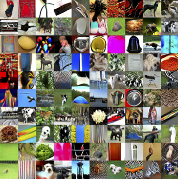
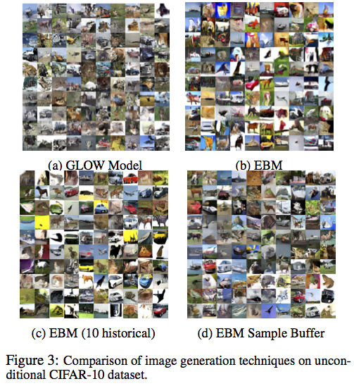
As for the results, one could say it rivals GANs, or one could say it falls short. The authors mainly experimented on CIFAR-10 and ImageNet. These two datasets are notoriously difficult, and even standard GANs often fail to generate well. From the result images, it can indeed compete with most GANs and clearly outperforms Glow on CIFAR-10. The reason I say it might fall short is that it feels a bit too reliant on specific tricks and lacks elegance—for instance, the sampling idea derived from the Langevin equation feels somewhat uncertain to me, and the practice of maintaining a Buffer, while effective in practice, clearly has a very strong "engineering" flavor...

Reprinting: Please include the original address of this article: https://kexue.fm/archives/6612

For more details on reprinting, please refer to: "Scientific Space FAQ"