Optimization Algorithms from a Dynamics Perspective (IV): The Third Stage of GAN

Dynamical Systems

In our series “Optimization Algorithms from a Dynamics Perspective,” we view gradient descent as mathematically solving a dynamical system (i.e., a system of ordinary differential equations, or ODEs): \dot{\boldsymbol{\theta}} = - \nabla_{\boldsymbol{\theta}} L(\boldsymbol{\theta}) where L(\boldsymbol{\theta}) is the loss of the model and \boldsymbol{\theta} represents the parameters of the model. If randomness is considered, a noise term needs to be added, turning it into a stochastic differential equation. However, in this article, we do not consider randomness, as it does not affect our analysis of local convergence. Assuming the reader is familiar with this conversion, let’s discuss the process corresponding to GANs.

GAN is a min-max process; in other words, one side is gradient descent and the other is gradient ascent. Assuming \boldsymbol{\varphi} are the parameters of the discriminator and \boldsymbol{\theta} are the parameters of the generator, the dynamical system corresponding to GAN is: \begin{pmatrix}\dot{\boldsymbol{\varphi}}\\ \dot{\boldsymbol{\theta}}\end{pmatrix} = \begin{pmatrix} \nabla_{\boldsymbol{\varphi}} L(\boldsymbol{\varphi},\boldsymbol{\theta})\\ - \nabla_{\boldsymbol{\theta}} L(\boldsymbol{\varphi},\boldsymbol{\theta})\end{pmatrix} Of course, for more general GANs, sometimes the two L functions are slightly different: \begin{pmatrix}\dot{\boldsymbol{\varphi}}\\ \dot{\boldsymbol{\theta}}\end{pmatrix} = \begin{pmatrix} \nabla_{\boldsymbol{\varphi}} L_1(\boldsymbol{\varphi},\boldsymbol{\theta})\\ - \nabla_{\boldsymbol{\theta}} L_2(\boldsymbol{\varphi},\boldsymbol{\theta})\end{pmatrix} Regardless of which one it is, the two terms on the right side have opposite signs, and it is precisely this difference in signs that leads to difficulties in GAN training. We will gradually come to recognize this below.

Related Work

There have been many studies treating the optimization process of GANs as a (stochastic) dynamical system. Those I have read include “The Numerics of GANs”, “GANs Trained by a Two Time-Scale Update Rule Converge to a Local Nash Equilibrium”, “Gradient descent GAN optimization is locally stable”, and “Which Training Methods for GANs do actually Converge?”. This article is merely a summary of the work of these predecessors.

Among these papers, readers might be most familiar with the second one, as it proposed the TTUR training strategy for GANs and introduced FID as a performance metric. The theoretical basis of that paper also treats GAN optimization as the aforementioned stochastic dynamical system and cites a theorem from stochastic optimization to conclude that different learning rates can be used for the generator and discriminator (TTUR). The other papers directly treat GAN optimization as a deterministic dynamical system (ODEs) and use ODE analysis methods. Since the theoretical analysis and numerical solution of ODEs are quite mature, many ODE conclusions can be directly applied to GANs.

Dirac GAN

The ideas and results in this article mainly refer to “Which Training Methods for GANs do actually Converge?”. The main contributions of that paper are as follows:

1. Proposed the concept of Dirac GAN, which allows for a quick basic understanding of GAN behavior;

2. Completely analyzed the local convergence of WGAN with zero-centered gradient penalty (also known as WGAN-div);

3. Used WGAN with zero-centered gradient penalty to train 1024 \times 1024 faces and 256 \times 256 LSUN generation without the need for progressive training like PGGAN.

Due to experimental equipment limitations, we cannot easily replicate the third point, and the second point involves complex theoretical analysis that we will not discuss too much. Interested readers can read the original paper. This article mainly focuses on the first point: Dirac GAN.

The so-called Dirac GAN considers the performance of the GAN model under the condition that the true sample distribution has only one sample point. Assume the real sample point is the zero vector \boldsymbol{0}, and the fake sample is \boldsymbol{\theta}, which also represents the parameters of the generator. The discriminator uses the simplest linear model, i.e., D(\boldsymbol{x}) = \boldsymbol{x} \cdot \boldsymbol{\varphi} (before the activation function), where \boldsymbol{\varphi} represents the discriminator’s parameters. Dirac GAN considers whether the fake sample can eventually converge to the real sample in such a minimalist model—that is, whether \boldsymbol{\theta} can eventually converge to \boldsymbol{0}.

However, the original paper only considered the case where the sample point dimension is one-dimensional (i.e., \boldsymbol{0}, \boldsymbol{\theta}, \boldsymbol{\varphi} are all scalars). But the cases later in this article show that for some examples, a 1D Dirac GAN is insufficient to reveal its convergence behavior. In general, at least a 2D Dirac GAN is needed to better analyze the asymptotic convergence of a GAN.

Vanilla GAN

Vanilla GAN, also known as the original or standard GAN, refers to the GAN first proposed by Goodfellow. It has two forms: saturating and non-saturating. As an example, let’s analyze the commonly used non-saturating form: \begin{aligned} &\min_D \mathbb{E}_{\boldsymbol{x}\sim p(\boldsymbol{x})}[-\log D(\boldsymbol{x})]+\mathbb{E}_{\boldsymbol{x}\sim q(\boldsymbol{x})}[-\log (1-D(\boldsymbol{x}))]\\ &\min_G \mathbb{E}_{\boldsymbol{z}\sim q(\boldsymbol{z})}[-\log D(G(\boldsymbol{z}))] \end{aligned} Here p(\boldsymbol{x}) and q(\boldsymbol{x}) are the true and fake sample distributions, respectively, and q(\boldsymbol{z}) is the noise distribution. D(\boldsymbol{x}) is activated with a sigmoid. In the Dirac GAN setting, this is much simpler because the true sample is just one point at \boldsymbol{0}, so the discriminator loss has only one term, and the discriminator can be written as \boldsymbol{\theta} \cdot \boldsymbol{\varphi}, where \boldsymbol{\theta} is the fake sample or the generator. The result is: \begin{aligned} &\min_{\boldsymbol{\varphi}} -\log (1-\sigma(\boldsymbol{\theta}\cdot \boldsymbol{\varphi}))\\ &\min_{\boldsymbol{\theta}} -\log \sigma(\boldsymbol{\theta}\cdot \boldsymbol{\varphi}) \end{aligned} The corresponding dynamical system is: \begin{pmatrix}\dot{\boldsymbol{\varphi}}\\ \dot{\boldsymbol{\theta}}\end{pmatrix} = \begin{pmatrix} \nabla_{\boldsymbol{\varphi}} \log (1-\sigma(\boldsymbol{\theta}\cdot \boldsymbol{\varphi}))\\ \nabla_{\boldsymbol{\theta}} \log \sigma(\boldsymbol{\theta}\cdot \boldsymbol{\varphi})\end{pmatrix} = \begin{pmatrix} - \sigma(\boldsymbol{\theta}\cdot \boldsymbol{\varphi}) \boldsymbol{\theta}\\ (1 - \sigma(\boldsymbol{\theta}\cdot \boldsymbol{\varphi}))\boldsymbol{\varphi}\end{pmatrix} The equilibrium point of this dynamical system (where the right side equals 0) is \boldsymbol{\varphi}=\boldsymbol{\theta}=\boldsymbol{0}, meaning the fake sample has become the real sample. But the question is whether the system will eventually converge to the equilibrium point starting from an initial point.

To make a judgment, we assume the system has reached the vicinity of the equilibrium point, i.e., \boldsymbol{\varphi}\approx \boldsymbol{0}, \boldsymbol{\theta}\approx \boldsymbol{0}. Then we can perform an approximate linear expansion: \begin{pmatrix}\dot{\boldsymbol{\varphi}}\\ \dot{\boldsymbol{\theta}}\end{pmatrix} = \begin{pmatrix} - \sigma(\boldsymbol{\theta}\cdot \boldsymbol{\varphi}) \boldsymbol{\theta}\\ (1 - \sigma(\boldsymbol{\theta}\cdot \boldsymbol{\varphi}))\boldsymbol{\varphi}\end{pmatrix} \approx \begin{pmatrix} - \boldsymbol{\theta} / 2\\ \boldsymbol{\varphi} / 2\end{pmatrix} Ultimately, we approximately have: \ddot{\boldsymbol{\theta}}\approx - \boldsymbol{\theta} / 4 Students who have studied ODEs know that this is one of the simplest linear ODEs. As long as the initial value is not \boldsymbol{0}, its solution is a periodic solution, meaning that the characteristic \boldsymbol{\theta}\to \boldsymbol{0} will not occur. In other words, for the non-saturating Vanilla GAN, even if the model initialization is already quite close to the equilibrium point, it will never converge to it but will oscillate around it. Numerical simulation results further prove this point.

In fact, similar results appear in any form of f-GAN. That is, all GANs based on f-divergence (excluding regularization terms) have the same problem: they will slowly approach the vicinity of the equilibrium point and eventually just oscillate around it, unable to fully converge.

To repeat the logic: we know that the theoretical equilibrium point of the system is indeed what we want, but starting from an arbitrary initial value (equivalent to model initialization), whether it can eventually reach the theoretical equilibrium point after iteration (equivalent to ideally completing GAN training) is not an obvious result. At the very least, a linear expansion near the equilibrium point is needed to analyze its convergence, which is the so-called local asymptotic convergence behavior.

WGAN

f-GAN has failed; what about WGAN? Can it converge to the ideal equilibrium point?

The general form of WGAN is: \min_G \max_{D, \Vert D\Vert_L\leq 1} \mathbb{E}_{\boldsymbol{x}\sim p(\boldsymbol{x})}[D(\boldsymbol{x})] - \mathbb{E}_{\boldsymbol{z}\sim q(\boldsymbol{z})}[D(G(\boldsymbol{z}))] Corresponding to Dirac GAN, D(\boldsymbol{x})=\boldsymbol{x}\cdot \boldsymbol{\varphi}, and \Vert D\Vert_L\leq 1 can be guaranteed by \Vert \boldsymbol{\varphi}\Vert=1 (where \Vert\cdot\Vert is the l_2 norm). In other words, D(\boldsymbol{x}) with the L-constraint is D(\boldsymbol{x})=\boldsymbol{x}\cdot \boldsymbol{\varphi} / \Vert\boldsymbol{\varphi}\Vert. Then the Dirac GAN corresponding to WGAN is: \min_{\boldsymbol{\theta}}\max_{\boldsymbol{\varphi}} \frac{-\boldsymbol{\theta}\cdot \boldsymbol{\varphi}}{\Vert\boldsymbol{\varphi}\Vert} The corresponding dynamical system is: \begin{pmatrix}\dot{\boldsymbol{\varphi}}\\ \dot{\boldsymbol{\theta}}\end{pmatrix} = \begin{pmatrix} \nabla_{\boldsymbol{\varphi}} (-\boldsymbol{\theta}\cdot \boldsymbol{\varphi} / \Vert \boldsymbol{\varphi}\Vert)\\ \nabla_{\boldsymbol{\theta}} (\boldsymbol{\theta}\cdot \boldsymbol{\varphi} / \Vert \boldsymbol{\varphi}\Vert)\end{pmatrix} = \begin{pmatrix} -\boldsymbol{\theta} / \Vert \boldsymbol{\varphi}\Vert + (\boldsymbol{\theta}\cdot \boldsymbol{\varphi})\boldsymbol{\varphi} / \Vert \boldsymbol{\varphi}\Vert^3\\ \boldsymbol{\varphi} / \Vert \boldsymbol{\varphi}\Vert\end{pmatrix} We are mainly concerned with whether \boldsymbol{\theta} will tend to \boldsymbol{0}. We could introduce a linear expansion similar to the previous section, but since \Vert \boldsymbol{\varphi}\Vert is in the denominator, discussion becomes difficult. The most straightforward way is to solve this system numerically. The results are as follows:

As can be seen, the result is still oscillation near the equilibrium point, failing to reach it. This result indicates that WGAN (and naturally including Spectral Normalization) does not have local convergence. Even if it reaches the vicinity of the equilibrium point, it still cannot accurately land on it.

(Note: A brief analysis shows that if only a 1D Dirac GAN is considered, it will be impossible to analyze the WGAN in this section and the GAN-QP later. This is the limitation of considering only the 1D case.)

WGAN-GP

One might wonder, we just discussed WGAN, why discuss WGAN-GP?

In fact, from an optimization perspective, the WGAN mentioned earlier and WGAN-GP are two different types of models. The previous WGAN refers to adding an L-constraint to the discriminator beforehand (such as Spectral Normalization) and then performing adversarial learning; WGAN-GP here refers to not adding an L-constraint to the discriminator but instead forcing the discriminator to have an L-constraint through a Gradient Penalty term. There are two types of gradient penalties discussed here. The first is the “1-centered gradient penalty” proposed in “Improved Training of Wasserstein GANs”, and the second is the “0-centered gradient penalty” advocated in papers like “Wasserstein Divergence for GANs” and “Which Training Methods for GANs do actually Converge?”. Below we will compare the different performances of these two gradient penalties.

The general form of gradient penalty is: \begin{aligned} &\min_{D} \mathbb{E}_{\boldsymbol{x}\sim q(\boldsymbol{x})}[D(\boldsymbol{x})] - \mathbb{E}_{\boldsymbol{x}\sim p(\boldsymbol{x})}[D(\boldsymbol{x})] + \lambda \mathbb{E}_{\boldsymbol{x}\sim r(\boldsymbol{x})}\left[(\left\Vert\nabla_{\boldsymbol{x}}D(\boldsymbol{x})\right\Vert - c)^2\right]\\ &\min_{G} \mathbb{E}_{\boldsymbol{z}\sim q(\boldsymbol{z})}[-D(G(\boldsymbol{z}))] \end{aligned} where c=0 or c=1, and r(\boldsymbol{x}) is some derived distribution of p(\boldsymbol{x}) and q(\boldsymbol{x}), usually taken as the real sample distribution, fake sample distribution, or an interpolation of the two.

For Dirac GAN: \nabla_{\boldsymbol{x}}D(\boldsymbol{x}) = \nabla_{\boldsymbol{x}}(\boldsymbol{x}\cdot\boldsymbol{\varphi})=\boldsymbol{\varphi} This means it has nothing to do with \boldsymbol{x}, so how r(\boldsymbol{x}) is chosen does not affect the result. Therefore, the Dirac GAN version of WGAN-GP is: \begin{aligned} &\min_{\boldsymbol{\varphi}} \boldsymbol{\theta}\cdot\boldsymbol{\varphi} + \lambda (\left\Vert \boldsymbol{\varphi}\right\Vert - c)^2\\ &\min_{\boldsymbol{\theta}} -\boldsymbol{\theta}\cdot\boldsymbol{\varphi} \end{aligned} The corresponding dynamical system is: \begin{pmatrix}\dot{\boldsymbol{\varphi}}\\ \dot{\boldsymbol{\theta}}\end{pmatrix} = \begin{pmatrix} \nabla_{\boldsymbol{\varphi}} (-\boldsymbol{\theta}\cdot\boldsymbol{\varphi} - \lambda (\left\Vert \boldsymbol{\varphi}\right\Vert - c)^2)\\ \nabla_{\boldsymbol{\theta}} (\boldsymbol{\theta}\cdot\boldsymbol{\varphi})\end{pmatrix} = \begin{pmatrix} -\boldsymbol{\theta} - 2\lambda (1 - c / \Vert \boldsymbol{\varphi}\Vert) \boldsymbol{\varphi} \\ \boldsymbol{\varphi} \end{pmatrix} Next, we observe whether \boldsymbol{\theta} tends to \boldsymbol{0} when c=0 and c=1. When c=0, it is actually a linear system of ODEs that can be solved analytically, but when c=1, it is more complex. Therefore, for simplicity, we still use numerical solutions:

The figures above show the different behaviors of gradient penalty for c=0 and c=1 under the same initial conditions. All other parameters are the same. It can be seen that after adding the “1-centered gradient penalty,” Dirac GAN does not asymptotically converge to the origin but instead converges to a circle; however, adding the “0-centered gradient penalty” can achieve convergence. This indicates that the early gradient penalty terms indeed had some flaws, and the “0-centered gradient penalty” has better convergence behavior. Although the above analysis was only for Dirac GAN, the conclusion is representative, as the general proof of the superiority of the 0-centered gradient penalty is given in “Which Training Methods for GANs do actually Converge?” and has been experimentally verified.

GAN-QP

Finally, let’s analyze the performance of the GAN-QP I proposed. Compared to WGAN-GP, GAN-QP replaces the gradient penalty with a quadratic difference penalty and provides some proofs. Compared to gradient penalty, the main advantage of the difference penalty is faster computation.

GAN-QP can have multiple forms. A basic form is: \begin{aligned} &\min_{D} \mathbb{E}_{\boldsymbol{x}_r\sim p(\boldsymbol{x}_r),\boldsymbol{x}_f\sim q(\boldsymbol{x}_f)}\left[D(\boldsymbol{x}_f) - D(\boldsymbol{x}_r) + \frac{(D(\boldsymbol{x}_f) - D(\boldsymbol{x}_r))^2}{2\lambda \Vert \boldsymbol{x}_f - \boldsymbol{x}_r\Vert}\right]\\ &\min_{G} \mathbb{E}_{\boldsymbol{z}\sim q(\boldsymbol{z})}[-D(G(\boldsymbol{z}))] \end{aligned} The corresponding Dirac GAN is: \begin{aligned} &\min_{\boldsymbol{\varphi}} \boldsymbol{\theta}\cdot\boldsymbol{\varphi} + \frac{(\boldsymbol{\theta}\cdot\boldsymbol{\varphi})^2}{2\lambda \Vert \boldsymbol{\theta}\Vert}\\ &\min_{\boldsymbol{\theta}} -\boldsymbol{\theta}\cdot\boldsymbol{\varphi} \end{aligned} The corresponding dynamical system is: \begin{pmatrix}\dot{\boldsymbol{\varphi}}\\ \dot{\boldsymbol{\theta}}\end{pmatrix} = \begin{pmatrix} \nabla_{\boldsymbol{\varphi}} (-\boldsymbol{\theta}\cdot\boldsymbol{\varphi} - (\boldsymbol{\theta}\cdot\boldsymbol{\varphi})^2 / (2\lambda \Vert \boldsymbol{\theta}\Vert))\\ \nabla_{\boldsymbol{\theta}} (\boldsymbol{\theta}\cdot\boldsymbol{\varphi})\end{pmatrix} = \begin{pmatrix} -\boldsymbol{\theta} - (\boldsymbol{\theta}\cdot\boldsymbol{\varphi})\boldsymbol{\theta}/(\lambda \Vert \boldsymbol{\theta}\Vert)\\ \boldsymbol{\varphi} \end{pmatrix} The numerical results are shown below (first image):

Unfortunately, like most GANs, GAN-QP also oscillates.

L2 Regularization

The first solution is to consider adding an L2 regularization term to the discriminator’s weights (for any GAN). As mentioned above, the zero-centered gradient penalty is indeed good, but unfortunately, gradient penalty is too slow. If you are unwilling to add gradient penalty, you can consider adding an L2 regularization term.

Intuitively, GANs fall into oscillation near the equilibrium point, reaching a dynamic balance (periodic solution rather than a static solution). An L2 regularization term will force the discriminator’s weights toward zero, which may break this balance, as shown in the second image above. In my own GAN experiments, adding a slight L2 regularization term to the discriminator makes the model convergence more stable and slightly improves the results. (Of course, the weight of the regularization term needs to be adjusted according to the model.)

Weight Moving Average

In fact, the most powerful technique for mitigating this problem is Exponential Moving Average (EMA) of weights.

The basic concept of weight moving average was introduced in “Making Keras Cooler: Intermediate Variables, Weight Sliding, and Safe Generators.”. For its application in GANs, it is not difficult to understand because it can be observed that although most GANs eventually oscillate, the center of their oscillation is the equilibrium point! So the solution is simple: directly average the points on the oscillation trajectory to obtain an approximate oscillation center, thereby obtaining a solution closer to the equilibrium point (and thus higher quality)!

The improvement brought by weight moving average is very significant. The following figures compare the generation effects of O-GAN with and without weight moving average:

As can be seen, weight moving average brings a qualitative improvement to the generation results. The larger the decay rate, the smoother the generation results, but at the same time, some details will be lost; the smaller the decay rate, the more details are preserved, but naturally, extra noise may also be retained. Most mainstream GANs now use weight moving average, typically with a decay rate of 0.999.

By the way, in ordinary supervised training models, weight moving average can also generally bring an improvement in convergence speed. For example, the figure below shows the training curves of a ResNet20 model on CIFAR-10 with and without weight moving average, trained throughout with the Adam optimizer, a constant learning rate of 0.001, and an EMA decay rate of 0.9999:

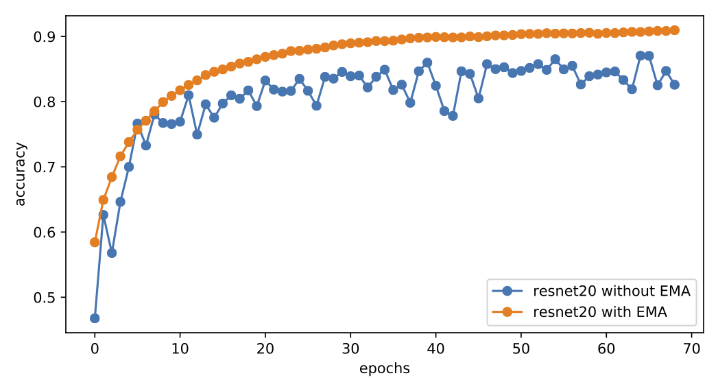
It can be seen that after adding weight moving average, the model converges to 90%+ accuracy in a very stable and fast manner, whereas without it, the model accuracy oscillates around 86%. This indicates that oscillation phenomena similar to those in GANs are common in deep learning training, and higher-quality models can be obtained through weight averaging.