Today, we introduce a very "brutal" model: the Invertible ResNet.
Why can a model be described as "brutal"? Naturally, it is because it is indeed very aggressive: it synthesizes many mathematical techniques to forcefully transform a conventional ResNet model into an invertible one (under certain constraints)!
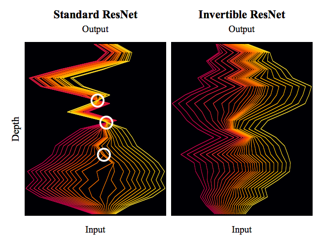
The model comes from the paper "Invertible Residual Networks", which was previously reported by JiQiZhi (Machine Heart). In this article, we will briefly appreciate its principles and content.
Bits of Invertible Models
Why study Invertible ResNet models? What are the benefits? Has no one studied this before?
The Benefits of Invertibility
What does invertibility mean?
It means it is information-lossless. It means it might be used to create better classification networks, or it can be used directly as a generative model via maximum likelihood. Furthermore, thanks to the powerful capabilities of ResNet, it might perform better than previous models like Glow. In short, if a model is invertible, the cost of inversion is low, and the fitting ability is strong, then it has a wide range of applications (classification, density estimation, generation tasks, etc.).
The Invertible ResNet introduced in this article basically satisfies these requirements. Its inversion is relatively simple, and it essentially does not change the fitting capability of ResNet. Therefore, I believe it deserves to be called a "beautiful" model.
Limitations of Old Models
Research on invertible models has a long history; they are known as "flow-based models." Representative models include NICE, RealNVP, and Glow. I have written articles introducing them, and there are also some autoregressive flow models. Besides being used for generative models, there is also research on using invertible models for classification tasks, with representative works being RevNet and i-RevNet.
The design philosophy of these flow models is basically the same: through clever design, the inverse transformation of each layer is made simple, and the Jacobian matrix is a triangular matrix, making the Jacobian determinant easy to calculate. Such models are theoretically elegant and beautiful, but they have a serious problem: because the inverse transformation must be simple and the Jacobian determinant easy to calculate, the non-linear transformation capability of each layer is very weak. In fact, in models like Glow, only half of the variables are transformed in each layer. To ensure sufficient fitting capability, the model must be stacked very deep (for example, for 256 \times 256 face generation, the Glow model stacks about 600 convolutional layers with 200 million parameters), resulting in massive computational costs.
Directly Tackling the Residual Model
The Invertible ResNet this time is different from previous flow models. It simply adds some constraints to the ordinary ResNet structure to make the model invertible, effectively retaining the basic structure and most of the fitting capability of ResNet. In this way, our previous experience in designing ResNets can still be applied, and the model no longer needs to stack convolutions as desperately as Glow.
Of course, this comes at a price. Because there is no special design, we need relatively "brutal" methods to obtain its inverse function and Jacobian determinant. Therefore, this Invertible ResNet is beautiful, but also very brutal—it can be called the "ultimate brutal aesthetics."
The "Three Elements" of Invertibility
The basic module of a ResNet model is: y = x + g(x) \triangleq F(x) \label{eq:resnet} In other words, instead of using a neural network to fit y, we now use it to fit y - x, where x and y are vectors (tensors). The benefit of this is that gradients do not vanish easily, allowing for the training of deep networks and multi-channel information transmission. Invertibility means that x + g(x) is a one-to-one mapping, meaning each x has only one corresponding y, and vice versa. In theory, we can solve for the inverse function x = h(y).
I won’t go into too much background, but I should clarify one point: the generalized ResNet we use in classification problems allows for dimension changes via 1 \times 1 convolutions, but the ResNet here refers to a ResNet that does not change dimensions—that is, the sizes of x and y remain the same.
For a model claiming to be "invertible," three questions must be answered:
1. When is it invertible?
2. What is the inverse function?
3. How is the Jacobian determinant calculated?
In terms of difficulty, these three questions are progressive. Of course, if you only care about classification, then only the first point needs to be guaranteed; if you care about reconstructing images, you need the second point; if you want to use maximum likelihood to train a generative model like Glow, you need the third point.
Following the logic of the original paper, let’s solve these three problems (the "three main courses") one by one in a brutal feast.
When is it Invertible?
The first course is relatively the easiest to digest among the three, though "relatively" is the keyword—it still involves some basic knowledge of functional analysis. (Wait, don’t run away yet!)
Since [eq:resnet] is the basic module of ResNet, we only need to ensure that each module is invertible. A sufficient condition for [eq:resnet] to be invertible is: \text{Lip}(g) < 1 where \text{Lip}(g) \triangleq \max_{x_1 \neq x_2} \frac{\|g(x_1) - g(x_2)\|_2}{\|x_1 - x_2\|_2} is the Lipschitz norm of function g. In other words, if the Lipschitz norm of g is less than 1, [eq:resnet] is guaranteed to be invertible.
So when is the Lipschitz norm of g less than 1? Since g is a neural network, whether it uses convolutions or fully connected layers, it is composed of matrix operations and activation functions. A representative structure is: \text{Activation}(Wx + b) By the chain rule, a sufficient condition for "the Lipschitz norm of g to be less than 1" is that "the Lipschitz norm of the Activation is no more than 1" and "the Lipschitz norm of Wx + b is less than 1." Since the Activation is just a scalar function, "Lipschitz norm no more than 1" simply means its derivative does not exceed 1. Most commonly used activation functions (sigmoid, tanh, ReLU, ELU, Swish, etc.) satisfy this, so we don’t need to worry about it. "The Lipschitz norm of Wx + b is less than 1" means the Lipschitz norm of matrix W is less than 1.
The Lipschitz norm of matrix W is actually its "spectral norm," denoted as \text{Lip}(W) or \|W\|_2. Where have we seen the spectral norm of a matrix before? We discussed it in the article "Lipschitz Constraints in Deep Learning: Generalization and Generative Models". Combining these, the conclusion is:
By performing spectral normalization on all kernel weights W of model g and then multiplying by a coefficient c where 0 < c < 1 (i.e., W \leftarrow c W / \|W\|_2), we can make x + g(x) invertible.
What is the Inverse Function?
Why does this make it invertible? The proof process directly answers the second question. That is, we solve for the inverse function directly, which reveals the conditions for invertibility.
If y = x + g(x) is invertible, we want to find the inverse function x = h(y), which is essentially solving a system of non-linear equations. For simplicity, consider the iteration: x_{n+1} = y - g(x_n) \label{eq:nidiedai} Clearly, the sequence \{x_n\} depends on y. Once \{x_n\} converges to a fixed function: \lim_{n \to \infty} x_n(y) = \hat{h}(y) then we have \hat{h}(y) = y - g(\hat{h}(y)), which means \hat{h}(y) is the x = h(y) we seek.
In other words, if the iteration [eq:nidiedai] converges, the result is the inverse function of x + g(x). So we only need to determine when [eq:nidiedai] converges. This is where the condition \text{Lip}(g) < 1 comes in. We have: \forall x_1, x_2, \quad \|g(x_1) - g(x_2)\|_2 \leq \text{Lip}(g) \|x_1 - x_2\|_2 Therefore: \begin{aligned} \|x_{n+1} - x_n\|_2 &= \|g(x_n) - g(x_{n-1})\|_2 \\ &\leq \text{Lip}(g) \|x_n - x_{n-1}\|_2 \\ &= \text{Lip}(g) \|g(x_{n-1}) - g(x_{n-2})\|_2 \\ &\leq \text{Lip}(g)^2 \|x_{n-1} - x_{n-2}\|_2 \\ &\dots \\ &\leq \text{Lip}(g)^n \|x_1 - x_0\|_2 \\ \end{aligned} As we can see, the sufficient condition for \|x_{n+1} - x_n\|_2 \to 0 is \text{Lip}(g) < 1.
Note: Simply stating \|x_{n+1} - x_n\|_2 \to 0 does not prove that the sequence \{x_n\} converges (e.g., the sequence \{\ln n\} satisfies this but diverges). To prove convergence when \text{Lip}(g) < 1, we need a bit more work.
For any positive integer k, consider \|x_{n+k} - x_n\|_2: \begin{aligned} \|x_{n+k} - x_n\|_2 &\leq \|x_{n+k} - x_{n+k-1}\|_2 + \dots + \|x_{n+1} - x_n\|_2 \\ &\leq \left(\text{Lip}(g)^{n+k-1} + \dots + \text{Lip}(g)^n\right) \|x_1 - x_0\|_2 \\ &= \frac{1 - \text{Lip}(g)^k}{1 - \text{Lip}(g)} \cdot \text{Lip}(g)^n \|x_1 - x_0\|_2 \\ &\leq \frac{\text{Lip}(g)^n}{1 - \text{Lip}(g)} \|x_1 - x_0\|_2 \end{aligned} \label{eq:cauchy} We have obtained an upper bound for \|x_{n+k} - x_n\|_2 that depends only on n and can be made arbitrarily small. This means for any \varepsilon > 0, we can find an n such that for any positive integer k, \|x_{n+k} - x_n\|_2 < \varepsilon. Such a sequence is called a Cauchy sequence, which must converge. Thus, we have proven the convergence of \{x_n\}.
Incidentally, in [eq:cauchy], as k \to \infty, we get: \|x^* - x_n\|_2 \leq \frac{\text{Lip}(g)^n}{1 - \text{Lip}(g)} \|x_1 - x_0\|_2 The convergence speed of this iterative algorithm is proportional to \text{Lip}(g)^n. Naturally, the smaller \text{Lip}(g) is, the faster it converges, but a smaller \text{Lip}(g) also weakens the model’s fitting ability. In the original paper, its range is 0.5 to 0.9.
In broader terms, this is the Banach Fixed Point Theorem in functional analysis, also known as the Contraction Mapping Theorem (since \text{Lip}(g) < 1, g is called a contraction mapping).
Thus, we have answered why \text{Lip}(g) < 1 makes x + g(x) invertible and provided the method for finding the inverse function—iterating [eq:nidiedai] to sufficient precision:
After normalization ensures x + g(x) is invertible, its inverse function is the fixed point of x_{n+1} = y - g(x_n). In numerical computation, one only needs to iterate for a certain number of steps until the precision requirement is met.
Finally, we have finished the second course.
How is the Jacobian Determinant Calculated?
Now we come to the most "hardcore" question: how to calculate the Jacobian determinant? To solve this, the authors synthesized mathematical analysis, matrix theory, probability theory, and statistical sampling, making it the "most brutal" of the courses.
First, why calculate the Jacobian determinant? As mentioned, this is only necessary for generative models. For details, please refer to the earliest introduction to flow models on this site: "Flow-based Models: Basic Concepts and Implementation of NICE". We know the Jacobian determinant is the determinant of the Jacobian matrix: J_F \triangleq \frac{\partial}{\partial x}(x + g(x)) = I + \frac{\partial g}{\partial x} \triangleq I + J_g Again, although I haven’t used boldface, g outputs a vector and x is a vector; \partial g / \partial x is the matrix of partial derivatives (the Jacobian matrix).
The Jacobian determinant is \det(J_F) = \det(I + J_g). However, in generative modeling, what we actually need is the "logarithm of the absolute value of the Jacobian determinant": \ln |\det(J_F)| = \ln |\det(I + J_g)| \equiv \ln \det(I + J_g) The last identity holds because \det(I + J_g) is always positive, so the absolute value can be removed. This can be proven, but it’s a detail; interested readers can check the references provided by the authors.
What next? Calculate the Jacobian determinant directly by definition? No, because the computational cost would be too high, and backpropagation would require calculating the derivative of the determinant, which is even more complex. The authors devised a tedious but effective solution using the identity (see "Appreciation of the Identity \det(\exp(A)) = \exp(\text{Tr}(A))"): \ln \det(\boldsymbol{B}) = \text{Tr}(\ln (\boldsymbol{B})) We get: \ln \det(I + J_g) = \text{Tr}(\ln (I + J_g)) If we can find \ln (I + J_g), we just need to find the trace (the sum of diagonal elements). How to find \ln (I + J_g)? Again, referring to the power series expansion: \ln (I + J_g) = \sum_{n=1}^{\infty}(-1)^{n-1}\frac{J_g^n}{n} \label{eq:duishujishu} Note that the condition for this series to converge is \|J_g\|_2 < 1, which is exactly \text{Lip}(g) < 1—the constraint for Invertible ResNet. It is perfectly self-consistent.
Now \ln (I + J_g) has become an infinite series. If we truncate it at n terms, the error is proportional to \text{Lip}(g)^N. Thus: \text{Tr}(\ln (I + J_g)) = \sum_{n=1}^{N}(-1)^{n-1}\frac{\text{Tr}(J_g^n)}{n} + \mathcal{O}\left(\text{Lip}(g)^N\right) \label{eq:det2tr}
Is the problem solved? The above formula requires calculating J_g^n. Since J_g is a matrix, calculating the n-th power is computationally expensive. So the authors thought:
Since analytical tools are exhausted, let’s use probability and statistics.
Assume p(u) is a multivariate distribution with mean 0 and a covariance matrix equal to the identity matrix (the standard normal distribution fits this). Then for any matrix A: \text{Tr}(A) = \mathbb{E}_{u \sim p(u)} [u^\top A u] Using the properties of zero mean and identity covariance, this can be proven directly from the definition. Then, the authors proposed a method that seems both "shameless and reasonable": for each iteration, just randomly sample one vector u from p(u) and assume u^\top A u is the trace \text{Tr}(A): \text{Tr}(\ln (I + J_g)) \approx \sum_{n=1}^{N}(-1)^{n-1}\frac{u^\top J_g^n u}{n}, \quad u \sim p(u) \label{eq:tr-caiyang}
Readers might object: shouldn’t we average over all vectors? Is one random sample enough? Actually, it is, for the following reasons:
Our optimization is based on Stochastic Gradient Descent (SGD), which inherently involves error. Sampling only one u adds error, but re-sampling a different u at each iteration helps cancel out the error over time.
More importantly, the log-Jacobian determinant is used as an additional loss term to prevent the model from collapsing. Simply put, it can be viewed as a regularization term, and a bit of error in regularization is acceptable.
Thus, the calculation of \text{Tr}(J_g^n) was solved by the authors with this brutal (yet effective) scheme. Note that: u^\top J_g^n u = u^\top J_g(\dots(J_g(J_g u))) So there is no need to compute J_g^n explicitly. Each step only requires a matrix-vector multiplication, and the results can be reused, significantly reducing the computational load.
In summary:
By using the power series expansion of the Jacobian matrix [eq:duishujishu], converting the determinant calculation into a trace calculation [eq:det2tr], and using probabilistic sampling [eq:tr-caiyang], the Jacobian determinant can be calculated most efficiently.
Experimental Results
Initially, I was attracted by the beautiful concept of "Invertible ResNet." But seeing this, I admit I’m intimidated—it truly lives up to the reputation of "hard-confronting ResNet." I originally thought about implementing a simple MNIST generation for fun, but after confirming the number of tricks and the sheer brutality involved, I gave up.
So, let’s just look at the experimental results from the original paper.
Toy Datasets
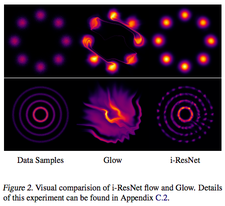
First is a synthetic Toy dataset, which involves fitting the distribution of points with regular patterns—a common experiment in GANs. As seen below, Invertible ResNet performs much better than Glow. Ultimately, I think this is because Invertible ResNet is a very symmetric model without much bias, whereas Glow is biased—it requires shuffling the input and splitting it in half, where the operations on the two halves are different, leading to asymmetry.
Classification Tasks
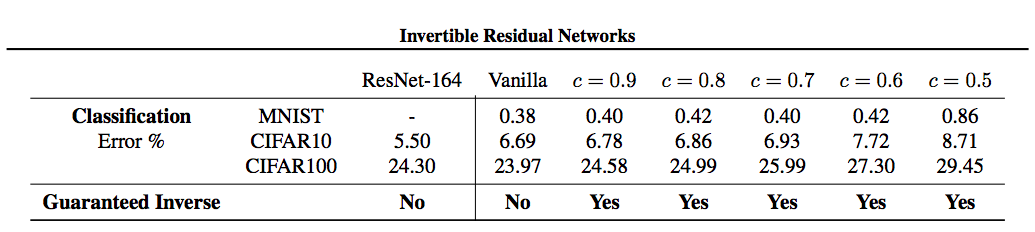
As we said at the beginning, since it is a type of ResNet, its most basic use is classification. The table below shows that using Invertible ResNet for classification yields very good results; the existence of the Lipschitz constraint does not significantly affect classification performance (where c in the table is \text{Lip}(g)).
Generative Model Experiments
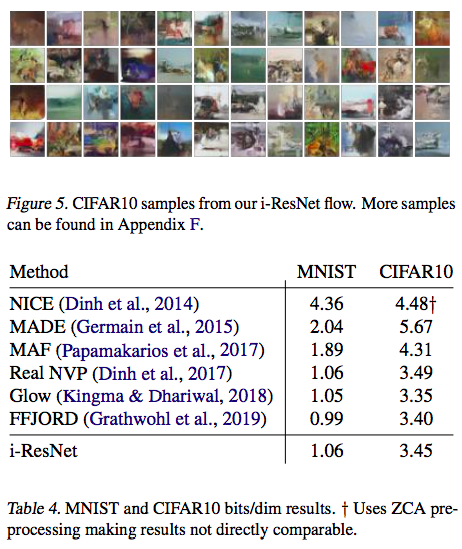
In fact, the flow model series is still far behind GANs in generating complex images, but quantitative comparisons between them are fine. The figure below also shows that Invertible ResNet is excellent as a flow-based generative model.
Conclusion
Directly tackling ResNet like this is truly a laborious task. Just interpreting it has been exhausting; I truly admire the authors’ mathematical prowess. Of course, the authors ultimately succeeded, and the joy of success must be immense. Overall, the entire work is brutal, but upon closer inspection, there is no sense of disharmony. Instead, there is a natural beauty to it, rather than a simple stacking of mathematical formulas.
The only problem is that the "hard-confrontation" process is quite complex, so widespread adoption would require good packaging, which often deters many. Another issue is that flow models, to ensure invertibility, cannot reduce dimensionality. Not reducing dimensionality inevitably leads to high computational costs—a contradictory point.
An interesting thought: for cases involving dimensionality reduction, could we create a model similar to a "pseudo-inverse" of a matrix to achieve an effect similar to Invertible ResNet? Non-square matrices can also have determinants (e.g., "Revisiting the Determinant of Non-Square Matrices"), so dimensionality-reducing transformations should also be able to produce a log-Jacobian determinant. It seems many aspects could be generalized.
Where will the flow model series go next? Let’s wait and see.
Reprinting: Please include the original link: https://kexue.fm/archives/6482
For more details on reprinting, please refer to: "Scientific Space FAQ"