From Wasserstein Distance and Duality Theory to WGAN

Cost Function

First, look at c(\boldsymbol{x},\boldsymbol{y}). It is a cost function representing the cost of transporting from \boldsymbol{x} to \boldsymbol{y}. A common choice is a power of the Euclidean distance: c(\boldsymbol{x},\boldsymbol{y}) = \Vert\boldsymbol{x}-\boldsymbol{y}\Vert^{\rho} In this case, we denote: \mathcal{W}_{\rho}[p,q]=\left(\mathcal{C}[p,q]\right)^{1/\rho} \mathcal{W}_{\rho}[p,q] is called the "Wasserstein distance" (more accurately, the "Wasserstein-\rho distance"). As we can see, the meaning of the optimal transport cost \mathcal{C}[p,q] is more general than the Wasserstein distance \mathcal{W}_{\rho}[p,q], so the subsequent derivations will primarily use \mathcal{C}[p,q]. When \rho=1, the optimal transport cost equals the corresponding Wasserstein distance.

Generally, the Euclidean distance \Vert\boldsymbol{x}-\boldsymbol{y}\Vert can be replaced by a more general distance, but the specific choice is not particularly important because many norms are equivalent. The equivalence of norms indicates that the resulting W-distances are essentially similar.

Cost Minimization

Next, look at \gamma. The condition \gamma\in \Pi[p,q] means: \int \gamma(\boldsymbol{x},\boldsymbol{y}) d\boldsymbol{y}=p(\boldsymbol{x})\quad\text{and}\quad\int \gamma(\boldsymbol{x},\boldsymbol{y}) d\boldsymbol{x}=q(\boldsymbol{y}) This means that \gamma is a joint distribution whose marginal distributions are the original p and q.

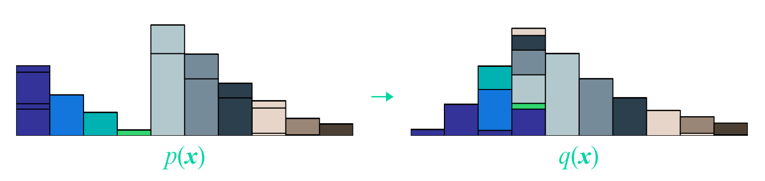
In fact, \gamma describes a transport plan. Without loss of generality, let p be the source distribution and q be the target distribution. p(\boldsymbol{x}) means that originally there is an amount p(\boldsymbol{x}) of goods at position \boldsymbol{x}, and q(\boldsymbol{x}) means the amount of goods to be stored at \boldsymbol{x} eventually. If p(\boldsymbol{x}) > q(\boldsymbol{x}), then part of the goods at \boldsymbol{x} must be moved elsewhere; conversely, if p(\boldsymbol{x}) < q(\boldsymbol{x}), then some goods must be moved from elsewhere to \boldsymbol{x}. And \gamma(\boldsymbol{x}, \boldsymbol{y}) means that an amount \gamma(\boldsymbol{x}, \boldsymbol{y})d\boldsymbol{x} is to be moved from \boldsymbol{x} to \boldsymbol{y}.

Finally, \inf denotes the infimum, which simply means taking the minimum. That is, from all possible transport plans, we want to find the plan that minimizes the total transport cost \iint \gamma(\boldsymbol{x},\boldsymbol{y}) c(\boldsymbol{x},\boldsymbol{y}) d\boldsymbol{x}d\boldsymbol{y}. The cost of this plan is the \mathcal{C}[p,q] we want to calculate. If we replace "goods" in the analogy with "soil," then the optimal transport cost is seeking the most labor-saving "earth-moving" plan. Therefore, the Wasserstein distance is often called the "Earth Mover’s Distance."

Finally, here is an adapted image from the aforementioned blog post to illustrate this "earth-moving" process:

Matrix Form

After analyzing the meaning term by term, let’s restate the problem completely. We are actually seeking the minimum of: \iint \gamma(\boldsymbol{x},\boldsymbol{y}) c(\boldsymbol{x},\boldsymbol{y}) d\boldsymbol{x}d\boldsymbol{y}\label{eq:ot-t} where c(\boldsymbol{x},\boldsymbol{y}) is given beforehand, and this minimum must satisfy the following constraints: \int \gamma(\boldsymbol{x},\boldsymbol{y}) d\boldsymbol{y}=p(\boldsymbol{x}),\quad\int \gamma(\boldsymbol{x},\boldsymbol{y}) d\boldsymbol{x}=q(\boldsymbol{y}),\quad \gamma(\boldsymbol{x},\boldsymbol{y})\geq 0\label{eq:ot-c}

Looking closely at Equation [eq:ot-t], and considering that integration is just the limit form of summation, we can discretize \gamma(\boldsymbol{x},\boldsymbol{y}) and c(\boldsymbol{x},\boldsymbol{y}) and view them as very long (column) vectors \boldsymbol{\Gamma} and \boldsymbol{C}: \boldsymbol{\Gamma}=\begin{pmatrix} \gamma(\boldsymbol{x}_1, \boldsymbol{y}_1) \\ \gamma(\boldsymbol{x}_1, \boldsymbol{y}_2) \\ \vdots \\ \hline \gamma(\boldsymbol{x}_2, \boldsymbol{y}_1) \\ \gamma(\boldsymbol{x}_2, \boldsymbol{y}_2) \\ \vdots \\ \hline \vdots \\ \hline \gamma(\boldsymbol{x}_n, \boldsymbol{y}_1) \\ \gamma(\boldsymbol{x}_n, \boldsymbol{y}_2) \\ \vdots \\ \hline \vdots \\ \end{pmatrix},\quad \boldsymbol{C}=\begin{pmatrix} c(\boldsymbol{x}_1, \boldsymbol{y}_1) \\ c(\boldsymbol{x}_1, \boldsymbol{y}_2) \\ \vdots \\ \hline c(\boldsymbol{x}_2, \boldsymbol{y}_1) \\ c(\boldsymbol{x}_2, \boldsymbol{y}_2) \\ \vdots \\ \hline \vdots \\ \hline c(\boldsymbol{x}_n, \boldsymbol{y}_1) \\ c(\boldsymbol{x}_n, \boldsymbol{y}_2) \\ \vdots \\ \hline \vdots \\ \end{pmatrix}\label{eq:lp-ot-t1}

So Equation [eq:ot-t] is equivalent to multiplying the corresponding positions of \boldsymbol{\Gamma} and \boldsymbol{C} and then summing them up. Isn’t this just the inner product \langle\boldsymbol{\Gamma},\boldsymbol{C}\rangle?

If you haven’t understood this yet, please stare at Equation [eq:ot-t] for a while longer, imagining the process of discretizing \boldsymbol{x}, \boldsymbol{y} into intervals and thinking about the definition of an integral. It shouldn’t be hard to grasp. If you have understood it, then it’s easy: we can also view the constraints [eq:ot-c] this way. View p(\boldsymbol{x}) and q(\boldsymbol{x}) as long vectors and concatenate them. View the integral as a sum. Then the constraints [eq:ot-c] can be written in matrix form \boldsymbol{A}\boldsymbol{\Gamma}=\boldsymbol{b}: \underbrace{\left( \begin{array}{ccc|ccc|c|ccc|c} 1 & 1 & \dots & 0 & 0 & \dots & \dots & 0 & 0 & \dots & \dots \\ 0 & 0 & \dots & 1 & 1 & \dots & \dots & 0 & 0 & \dots & \dots \\ \vdots & \vdots & \ddots & \vdots & \vdots & \ddots & \ddots & \vdots & \vdots & \ddots & \ddots \\ 0 & 0 & \dots & 0 & 0 & \dots & \dots & 1 & 1 & \dots & \dots \\ \vdots & \vdots & \ddots & \vdots & \vdots & \ddots & \ddots & \vdots & \vdots & \ddots & \ddots \\ \hline 1 & 0 & \dots & 1 & 0 & \dots & \dots & 1 & 0 & \dots & \dots \\ 0 & 1 & \dots & 0 & 1 & \dots & \dots & 0 & 1 & \dots & \dots \\ \vdots & \vdots & \ddots & \vdots & \vdots & \ddots & \ddots & \vdots & \vdots & \ddots & \ddots \\ 0 & 0 & \dots & 0 & 0 & \dots & \dots & 0 & 0 & \dots & \dots \\ \vdots & \vdots & \ddots & \vdots & \vdots & \ddots & \ddots & \vdots & \vdots & \ddots & \ddots \\ \end{array} \right)}_{\Large\boldsymbol{A}}\,\, \underbrace{\begin{pmatrix} \gamma(\boldsymbol{x}_1, \boldsymbol{y}_1) \\ \gamma(\boldsymbol{x}_1, \boldsymbol{y}_2) \\ \vdots \\ \hline \gamma(\boldsymbol{x}_2, \boldsymbol{y}_1) \\ \gamma(\boldsymbol{x}_2, \boldsymbol{y}_2) \\ \vdots \\ \hline \vdots \\ \hline \gamma(\boldsymbol{x}_n, \boldsymbol{y}_1) \\ \gamma(\boldsymbol{x}_n, \boldsymbol{y}_2) \\ \vdots \\ \hline \vdots \\ \end{pmatrix}}_{\Large\boldsymbol{\Gamma}} \,\,=\,\, \underbrace{\begin{pmatrix} p(\boldsymbol{x}_1) \\ p(\boldsymbol{x}_2) \\ \vdots \\ p(\boldsymbol{x}_n) \\ \vdots \\ \hline q(\boldsymbol{y}_1) \\ q(\boldsymbol{y}_2) \\ \vdots \\ q(\boldsymbol{y}_n) \\ \vdots \\ \end{pmatrix}}_{\Large\boldsymbol{b}}\label{eq:lp-ot-t2}

Finally, do not forget \boldsymbol{\Gamma}\geq 0, which means every component of \boldsymbol{\Gamma} is greater than or equal to 0.

Linear Programming Problem

Now the problem can be described in one line: \min_{\boldsymbol{\Gamma}}\big\{\langle\boldsymbol{\Gamma},\boldsymbol{C}\rangle\,\big|\,\boldsymbol{A}\boldsymbol{\Gamma}=\boldsymbol{b},\,\boldsymbol{\Gamma}\geq 0\big\}\label{eq:lp-ot}

This is the problem of "<u>minimizing a linear function under linear constraints</u>," which is the linear programming problem we encountered in high school. It can be seen that although the original problem is complex, involving integrals and infimums, after rewriting, it is essentially a linear programming problem that is not difficult to understand (of course, "not difficult to understand" does not mean "easy to solve").

Weak Duality Form

In planning and optimization problems, the "dual form" is a very important concept. Generally, "duality" refers to a transformation that converts the original problem into an equivalent but seemingly different new problem: \text{Primal Problem}\quad\xrightarrow{\text{Dual Transformation}}\quad \text{New Problem} The reason "duality" is called "duality" is that applying the same form of transformation to the new problem usually restores the original problem: \text{New Problem}\quad\xrightarrow{\text{Dual Transformation}}\quad \text{Primal Problem} Thus, "duality" is like a mirror; the primal and new problems are like the "object" and the "image." Solving one problem is equivalent to solving the other. So we just look for whichever one is simpler.

Readers might wonder: what is the difference between "duality" and equivalent descriptions in mathematics like "contrapositive propositions"? There is no fundamental difference; simply put, both "duality" and "contrapositive propositions" are completely equivalent to the original proposition. However, "duality" looks very different from the primal proposition, whereas a "contrapositive" is merely a logical transformation. From a linear algebra perspective, "duality" is like the relationship between the "primal space" and the "dual space" (complementary space) in vector spaces.

Strong Duality Form

As mentioned, from a practical standpoint, weak duality is often enough. However, for readers interested in the complete theory, we will also argue for the "strong duality form." Readers only interested in WGAN itself may consider skipping this part.

The strong duality form is: \max_{\boldsymbol{y}}\big\{\boldsymbol{b}^{\top}\boldsymbol{y}\,\big|\,\boldsymbol{A}^{\top}\boldsymbol{y}\leq \boldsymbol{c}\big\} = \min_{\boldsymbol{x}}\big\{\boldsymbol{c}^{\top}\boldsymbol{x}\,\big|\,\boldsymbol{A}\boldsymbol{x}=\boldsymbol{b},\,\boldsymbol{x}\geq 0\big\}\label{eq:strong-dual} Note that while weak duality holds for many optimization problems, strong duality does not necessarily hold. However, for linear programming, strong duality does hold.

Farkas Lemma

The proof of the strong duality form mainly uses a conclusion called the "Farkas Lemma":

For a fixed matrix \boldsymbol{A}\in\mathbb{R}^{m\times n} and vector \boldsymbol{b}\in\mathbb{R}^m, exactly one of the following two options holds:

1. There exists \boldsymbol{x}\in \mathbb{R}^n with \boldsymbol{x}\geq 0 such that \boldsymbol{A}\boldsymbol{x}=\boldsymbol{b};
2. There exists \boldsymbol{y}\in \mathbb{R}^m such that \boldsymbol{A}^{\top}\boldsymbol{y}\leq 0 and \boldsymbol{b}^{\top}\boldsymbol{y} > 0.

What on earth? Transposes, inequalities? Can we speak in plain English?

Actually, this lemma has a very intuitive geometric explanation, though translating it into algebraic language is not simple. The starting point for the geometric explanation is to consider the following set of vectors: \big\{\boldsymbol{A}\boldsymbol{x}\big|\boldsymbol{x}\in \mathbb{R}^n\text{ and }\boldsymbol{x}\geq 0\big\} The meaning of this set is: if we view \boldsymbol{A} as a combination of n column vectors of dimension m: \boldsymbol{A}=(\boldsymbol{a}_1,\boldsymbol{a}_2,\dots,\boldsymbol{a}_n) then the set is actually all non-negative linear combinations of \boldsymbol{a}_1,\boldsymbol{a}_2,\dots,\boldsymbol{a}_n. What is this set? The answer is: a cone, as shown in the figure.

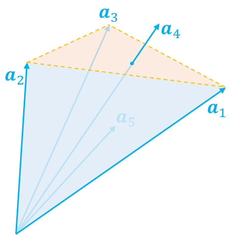
Now, if we pick an arbitrary vector \boldsymbol{b}, there are obviously only two possibilities, and exactly one must hold: 1. It is inside the cone (including the boundary); 2. It is outside the cone. (This is a tautology, but translating it into algebraic language makes it non-trivial.)

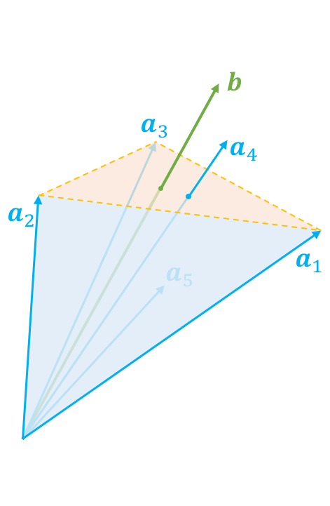
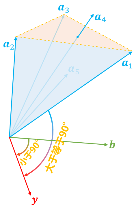
If it is inside the cone, then by the definition of the cone, it can be expressed as a non-negative linear combination of \boldsymbol{a}_1,\boldsymbol{a}_2,\dots,\boldsymbol{a}_n (the representation might not be unique), meaning there exists \boldsymbol{x}\geq 0 such that \boldsymbol{A}\boldsymbol{x}=\boldsymbol{b}. This is the first case.

What if it is outside the cone? How do we represent being outside? We could write the negation of the first case, but that’s not very useful. If vector \boldsymbol{b} is outside the cone, we can always find a "benchmark" vector \boldsymbol{y} such that the angle between it and each of \boldsymbol{a}_1,\boldsymbol{a}_2,\dots,\boldsymbol{a}_n is greater than or equal to 90 degrees. In vector notation, the inner products are all less than or equal to zero, i.e., (\boldsymbol{a}_1^{\top}\boldsymbol{y}, \boldsymbol{a}_2^{\top}\boldsymbol{y}, \dots, \boldsymbol{a}_n^{\top}\boldsymbol{y}) \leq 0, or written as a whole: \boldsymbol{A}^{\top}\boldsymbol{y} \leq 0. After finding this "benchmark," the angle between vector \boldsymbol{b} and the "benchmark" must be less than 90 degrees, i.e., \boldsymbol{b}^{\top}\boldsymbol{y} > 0. One being \geq 90^\circ and the other being < 90^\circ ensures that vector \boldsymbol{b} is outside the cone formed by all the vectors. This is the second case.

Of course, this is not a complete proof, but a heuristic guide. A complete proof would require carefully arguing why the non-negative linear combinations of these vectors form a cone. That is beyond the scope of this article. The characteristic of Farkas Lemma is the "either-or" nature. For example, to prove the second point is satisfied, one only needs to prove the first point is not satisfied, and vice versa. This is a transformation of the problem.

Duality of Transport Cost

Before the derivation, let’s recap the logic of this article: we introduced the definition of optimal transport cost \eqref{eq:ot} on which the W-distance depends. After analysis, we found it is actually a continuous version of a standard linear programming problem, with the transformation process being \eqref{eq:lp-ot-t1}, \eqref{eq:lp-ot-t2}, and \eqref{eq:lp-ot}. Therefore, we spent a significant portion of the article learning about linear programming and its duality, eventually reaching the conclusion \eqref{eq:strong-dual}.

Now, what we need to do is "reverse" the entire process—that is, find the continuous version corresponding to \eqref{eq:strong-dual} to find a dual expression for the optimal transport cost.

This process is not complicated. From the conclusion \eqref{eq:strong-dual} and Equation \eqref{eq:lp-ot}, we get: \min_{\boldsymbol{\Gamma}}\big\{\langle\boldsymbol{\Gamma},\boldsymbol{C}\rangle\,\big|\,\boldsymbol{A}\boldsymbol{\Gamma}=\boldsymbol{b},\,\boldsymbol{\Gamma}\geq 0\big\}=\max_{\boldsymbol{F}}\big\{\langle\boldsymbol{b},\boldsymbol{F}\rangle\,\big|\,\boldsymbol{A}^{\top}\boldsymbol{F}\leq \boldsymbol{C}\big\} Note that in Equation \eqref{eq:lp-ot-t2}, \boldsymbol{b} is composed of two parts, so we can similarly write \boldsymbol{F} as: \boldsymbol{F}=\begin{pmatrix} f(\boldsymbol{x}_1) \\ f(\boldsymbol{x}_2) \\ \vdots \\ f(\boldsymbol{x}_n) \\ \vdots \\ \hline g(\boldsymbol{y}_1) \\ g(\boldsymbol{y}_2) \\ \vdots \\ g(\boldsymbol{y}_n) \\ \vdots \\ \end{pmatrix} Now \langle\boldsymbol{b},\boldsymbol{F}\rangle can be written as: \langle\boldsymbol{b},\boldsymbol{F}\rangle=\sum_n p(\boldsymbol{x}_n) f(\boldsymbol{x}_n) + \sum_n q(\boldsymbol{x}_n) g(\boldsymbol{x}_n) Or the corresponding integral form: \langle\boldsymbol{b},\boldsymbol{F}\rangle=\int \big[p(\boldsymbol{x}) f(\boldsymbol{x}) + q(\boldsymbol{x}) g(\boldsymbol{x})\big]d\boldsymbol{x}

Don’t forget the constraint \boldsymbol{A}^{\top}\boldsymbol{F}\leq \boldsymbol{C}: \underbrace{\left( \begin{array}{ccccc|ccccc} 1 & 0 & \dots & 0 & \dots & 1 & 0 & \dots & 0 & \dots \\ 1 & 0 & \dots & 0 & \dots & 0 & 1 & \dots & 0 & \dots \\ \vdots & \vdots & \ddots & \vdots & \ddots & \vdots & \vdots & \ddots & \vdots & \ddots \\ \hline 0 & 1 & \dots & 0 & \dots & 1 & 0 & \dots & 0 & \dots \\ 0 & 1 & \dots & 0 & \dots & 0 & 1 & \dots & 0 & \dots \\ \vdots & \vdots & \ddots & \vdots & \ddots & \vdots & \vdots & \ddots & \vdots & \ddots \\ \hline \vdots & \vdots & \ddots & \vdots & \ddots & \vdots & \vdots & \ddots & \vdots & \ddots \\ \hline 0 & 0 & \dots & 1 & \dots & 1 & 0 & \dots & 0 & \dots \\ 0 & 0 & \ddots & 1 & \ddots & 0 & 1 & \ddots & 0 & \ddots \\ \vdots & \vdots & \ddots & \vdots & \ddots & \vdots & \vdots & \ddots & \vdots & \ddots \\ \hline \vdots & \vdots & \ddots & \vdots & \ddots & \vdots & \vdots & \ddots & \vdots & \ddots \\ \end{array} \right)}_{\Large\boldsymbol{A}^{\top}}\,\,\underbrace{\begin{pmatrix} f(\boldsymbol{x}_1) \\ f(\boldsymbol{x}_2) \\ \vdots \\ f(\boldsymbol{x}_n) \\ \vdots \\ \hline g(\boldsymbol{y}_1) \\ g(\boldsymbol{y}_2) \\ \vdots \\ g(\boldsymbol{y}_n) \\ \vdots \\ \end{pmatrix}}_{\Large\boldsymbol{F}}\,\,\leq\,\,\underbrace{\begin{pmatrix} c(\boldsymbol{x}_1, \boldsymbol{y}_1) \\ c(\boldsymbol{x}_1, \boldsymbol{y}_2) \\ \vdots \\ \hline c(\boldsymbol{x}_2, \boldsymbol{y}_1) \\ c(\boldsymbol{x}_2, \boldsymbol{y}_2) \\ \vdots \\ \hline \vdots \\ \hline c(\boldsymbol{x}_n, \boldsymbol{y}_1) \\ c(\boldsymbol{x}_n, \boldsymbol{y}_2) \\ \vdots \\ \hline \vdots \\ \end{pmatrix}}_{\Large \boldsymbol{C}} After substitution, we find that this massive matrix operation actually says one thing: \forall i,j,\,\,f(\boldsymbol{x}_i) + g(\boldsymbol{y}_j)\leq c(\boldsymbol{x}_i,\boldsymbol{y}_j) Or simply: \forall \boldsymbol{x},\boldsymbol{y},\,\,f(\boldsymbol{x}) + g(\boldsymbol{y})\leq c(\boldsymbol{x},\boldsymbol{y})

From Duality to WGAN

Finally, we are nearing the end. We have obtained a dual form for the optimal transport cost \eqref{eq:ot}: \mathcal{C}[p,q]=\max_{f,g}\Bigg\{\int \big[p(\boldsymbol{x}) f(\boldsymbol{x}) + q(\boldsymbol{x}) g(\boldsymbol{x})\big]d\boldsymbol{x} \,\Bigg|\,\, f(\boldsymbol{x}) + g(\boldsymbol{y})\leq c(\boldsymbol{x},\boldsymbol{y})\Bigg\} Notice that from f(\boldsymbol{x}) + g(\boldsymbol{y})\leq c(\boldsymbol{x},\boldsymbol{y}), we get: f(\boldsymbol{x}) + g(\boldsymbol{x})\leq c(\boldsymbol{x},\boldsymbol{x})=0 i.e., g(\boldsymbol{x}) \leq - f(\boldsymbol{x}), so we have: \begin{aligned}p(\boldsymbol{x}) f(\boldsymbol{x}) + q(\boldsymbol{x}) g(\boldsymbol{x})&\leq p(\boldsymbol{x}) f(\boldsymbol{x}) + q(\boldsymbol{x}) [-f(\boldsymbol{x})]\\ & = p(\boldsymbol{x}) f(\boldsymbol{x}) - q(\boldsymbol{x}) f(\boldsymbol{x})\end{aligned} This seems to suggest a conclusion: if g = -f, the maximum value will not be smaller than the original maximum. In fact, this conclusion is not entirely correct unless we specify that c(\boldsymbol{x},\boldsymbol{y}) is a distance (satisfying the triangle inequality). Further discussion on this detail can be found in the comments section of the original post. Next, we assume c(\boldsymbol{x},\boldsymbol{y}) is a distance function, which is exactly what WGAN considers. In this case, we can safely let g=-f, thus: \mathcal{C}[p,q]=\max_{f}\Bigg\{\int \big[p(\boldsymbol{x}) f(\boldsymbol{x}) - q(\boldsymbol{x}) f(\boldsymbol{x})\big]d\boldsymbol{x} \,\Bigg|\,\, f(\boldsymbol{x}) - f(\boldsymbol{y})\leq c(\boldsymbol{x},\boldsymbol{y})\Bigg\}\label{eq:ot-dual-u} This is the dual form of the optimal transport cost \eqref{eq:ot} we were looking for. Specifically, when c(\boldsymbol{x},\boldsymbol{y}) = \Vert \boldsymbol{x}-\boldsymbol{y}\Vert, we have \mathcal{C}[p,q] = \mathcal{W}_1[p,q], i.e.: \mathcal{W}_1[p,q]=\max_{f}\Bigg\{\int \big[p(\boldsymbol{x}) f(\boldsymbol{x}) - q(\boldsymbol{x}) f(\boldsymbol{x})\big]d\boldsymbol{x} \,\Bigg|\,\, f(\boldsymbol{x}) - f(\boldsymbol{y})\leq \Vert \boldsymbol{x}-\boldsymbol{y}\Vert\Bigg\}\label{eq:wd-dual-u} This is the W-distance used by WGAN, where the constraint is usually written as \Vert f\Vert_{L}\leq 1, known as the Lipschitz constraint. From this process, we can also see that theoretically, the c(\boldsymbol{x},\boldsymbol{y}) in WGAN can be a more general distance function, not just the Euclidean distance. However, since many distances are equivalent and the role of the distance here is just to add a constraint to the discriminator, choosing the Euclidean distance is sufficient.

Since p, q are probability distributions, we can write this in sampling form: \mathcal{W}_1[p,q]=\max_{f,\,\Vert f\Vert_{L}\leq 1}\mathbb{E}_{\boldsymbol{x}\sim p(\boldsymbol{x})}[f(\boldsymbol{x})] - \mathbb{E}_{\boldsymbol{x}\sim q(\boldsymbol{x})}[f(\boldsymbol{x})] This is the loss used by the WGAN discriminator. Naturally, the entire training process of WGAN is: \min_{G}\max_{f,\,\Vert f\Vert_{L}\leq 1}\mathbb{E}_{\boldsymbol{x}\sim p(\boldsymbol{x})}[f(\boldsymbol{x})] - \mathbb{E}_{\boldsymbol{z}\sim q(\boldsymbol{z})}[f(G(\boldsymbol{z}))] The long-awaited WGAN finally appears. The remaining issue is how to add the Lipschitz constraint, which can be referenced in: "Lipschitz Constraints in Deep Learning: Generalization and Generative Models".