Recently, by analyzing the dual space directly, I proposed an adversarial model framework called GAN-QP. Its main feature is that it can be theoretically proven to neither suffer from gradient vanishing nor require Lipschitz (L) constraints, thereby simplifying the construction and training of generative models.
GAN-QP is an adversarial framework, so theoretically, all original GAN tasks can be attempted using it. In the previous article "A GAN that doesn’t need L-constraints and won’t suffer from gradient vanishing, want to learn more?", we only experimented with standard random generation tasks. In this article, we explore the case involving both a generator and an encoder: BiGAN-QP.
BiGAN and BiGAN-QP
Note that this is BiGAN, not the recently popular BigGAN. BiGAN stands for Bidirectional GAN, proposed in the paper "Adversarial feature learning". Around the same time, a very similar paper titled "Adversarially Learned Inference" proposed a model called ALI, which is essentially the same as BiGAN. Generally speaking, they add an encoder to the standard GAN model, allowing the model to possess both the random generation capabilities of a normal GAN and the functionality of an encoder for extracting effective features. Applying the GAN-QP adversarial mode to BiGAN results in BiGAN-QP.
Without further ado, let’s look at the results first (left is the original image, right is the reconstruction):
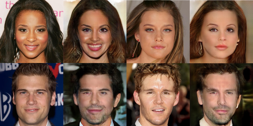
This was achieved by reducing a 256 \times 256 \times 3 image to a 256-dimensional vector and then reconstructing it. As we can see, the overall reconstruction effect is quite good, lacking the blurriness typical of standard autoencoders. While some details are missing—performing slightly worse compared to IntroVAE—this is a matter of model architecture and hyperparameter tuning, which are not my specialties. Regardless, this result demonstrates that BiGAN-QP is viable and effective.
The content of this article has been updated in the original GAN-QP paper: https://papers.cool/arxiv/1811.07296. Readers can download the latest version from arXiv.
Simple Derivation of BiGAN-QP
In fact, compared to GAN, the derivation of BiGAN is very simple. One only needs to replace the original single input x with dual inputs (x, z). Similarly, with the foundation of GAN-QP, BiGAN-QP is also straightforward. Specifically, the original GAN-QP was:
\begin{aligned} &T= \mathop{\text{argmax}}_T\, \mathbb{E}_{(x_r,x_f)\sim p(x_r)q(x_f)}\left[T(x_r,x_f)-T(x_f,x_r) - \frac{(T(x_r,x_f)-T(x_f,x_r))^2}{2\lambda d(x_r,x_f)}\right] \\ &G = \mathop{\text{argmin}}_G\,\mathbb{E}_{(x_r,x_f)\sim p(x_r)q(x_f)}\left[T(x_r,x_f)-T(x_f,x_r)\right] \end{aligned}
Now it becomes:
\begin{aligned} T&= \mathop{\text{argmax}}_T\, \mathbb{E}_{x\sim p(x), z\sim q(z)}\left[\Delta T - \frac{\Delta T^2}{2\lambda d\big(x,E(x);G(z),z\big)}\right] \\ G,E &= \mathop{\text{argmin}}_{G,E}\,\mathbb{E}_{x\sim p(x), z\sim q(z)}[\Delta T]\\ \Delta T &= T(x,E(x);G(z),z)-T(G(z),z;x,E(x)) \end{aligned}
Or a simplified version where we directly take \Delta T = T(x,E(x))-T(G(z),z). Theoretically, this is sufficient; this is BiGAN-QP.
However, in practice, it is difficult to learn a good bidirectional mapping this way because it is equivalent to searching for one bidirectional mapping out of infinite possibilities. Therefore, we need some "guidance terms." We use two MSE errors as guidance:
\begin{aligned} T&= \mathop{\text{argmax}}_T\, \mathbb{E}_{x\sim p(x), z\sim q(z)}\left[\Delta T - \frac{\Delta T^2}{2\lambda d\big(x,E(x);G(z),z\big)}\right] \\ G,E &= \mathop{\text{argmin}}_{G,E}\,\mathbb{E}_{x\sim p(x), z\sim q(z)}\Big[\Delta T + \beta_1 \Vert z - E(G(z))\Vert^2 + \beta_2 \Vert x - G(E(x))\Vert^2\Big]\\ \Delta T &= T(x,E(x))-T(G(z),z) \end{aligned}
The three loss terms for the generator are quite intuitive: \Delta T makes the generated images more realistic, \Vert z - E(G(z))\Vert^2 aims to reconstruct the latent variable space, and \Vert x - G(E(x))\Vert^2 aims to reconstruct the visible variable space. The latter two terms should not be too large, especially the last one, as a large value leads to image blurriness.
These two regularization terms can be seen as upper bounds on the mutual information between G(z) and z, and between x and E(x). From an information perspective, these terms encourage the mutual information between x and z to be as large as possible. Related discussions can be found in the InfoGAN paper; these terms imply that this model also belongs to the InfoGAN family. Thus, more completely, this should be called a Bi-Info-GAN-QP.
Mutual information terms can stabilize the GAN training process to some extent and reduce the possibility of mode collapse, because if the model collapses, the mutual information will not be high. In other words, if the model collapses, reconstruction becomes unlikely, and the reconstruction loss will be very large.
Experiments show that making a few small adjustments yields even better results. This adjustment stems from the fact that the two MSE terms, when coupled, are still too powerful (the loss values might not be large, but the gradients are), causing the model to still tend toward generating blurry images. Therefore, we need to stop half of the gradients, changing the formulation to:
\begin{aligned} T&= \mathop{\text{argmax}}_T\, \mathbb{E}_{x\sim p(x), z\sim q(z)}\left[\Delta T - \frac{\Delta T^2}{2\lambda d\big(x,E(x);G(z),z\big)}\right] \\ G,E &= \mathop{\text{argmin}}_{G,E}\,\mathbb{E}_{x\sim p(x), z\sim q(z)}\Big[\Delta T + \beta_1 \Vert z - E(G_{ng}(z))\Vert^2 + \beta_2 \Vert x - G(E_{ng}(x))\Vert^2\Big]\\ \Delta T &= T(x,E(x))-T(G(z),z) \end{aligned}
G_{ng} and E_{ng} refer to forcing the gradients of these parts to be zero. Most frameworks have this operator; you can call it directly. This is the final BiGAN-QP model used in this article.
Code and Results
The code has been added to GitHub: https://github.com/bojone/gan-qp/tree/master/bigan-qp
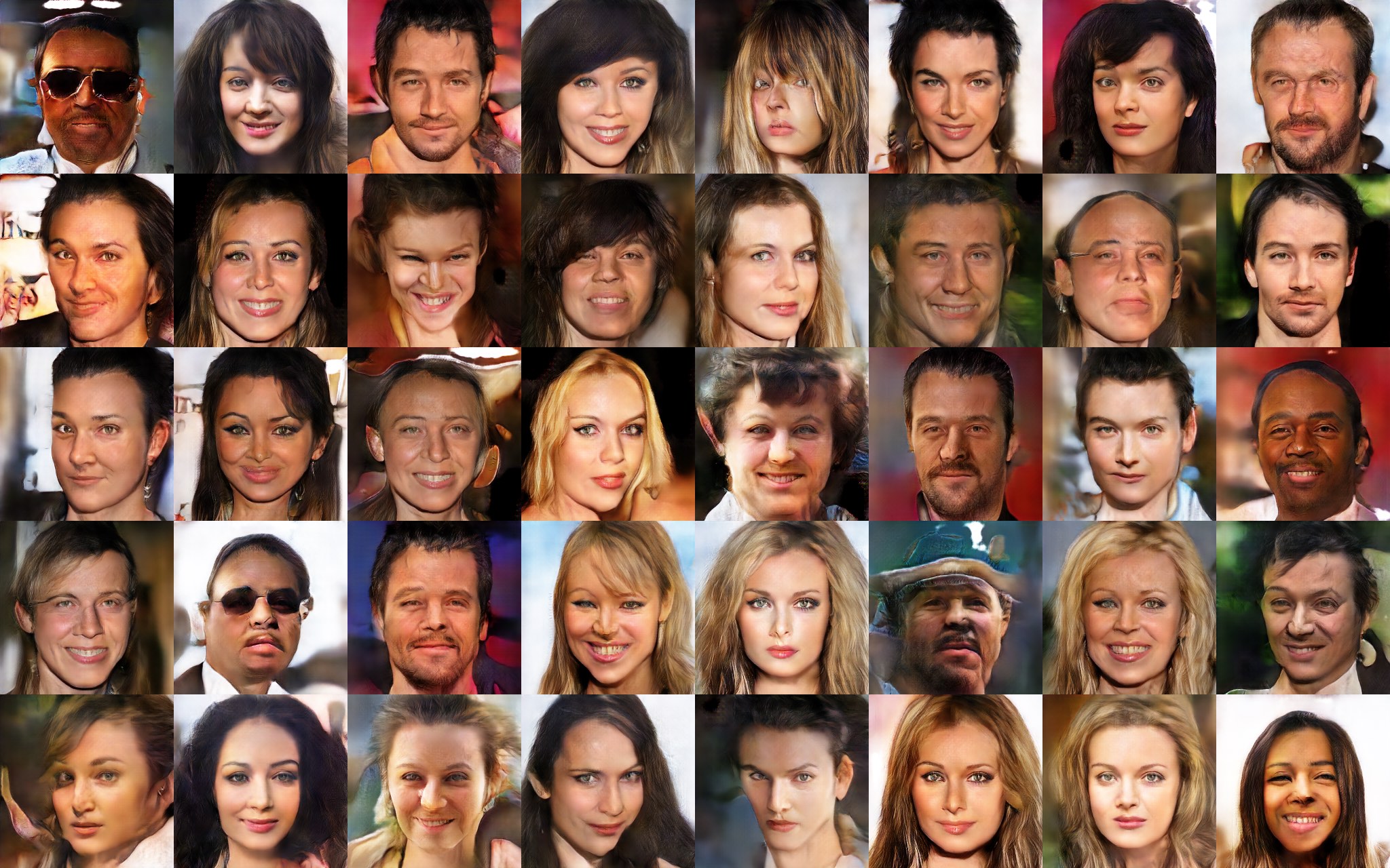
Here are some more results. First, randomly generated images:
Reconstruction images (left is original, right is reconstruction):
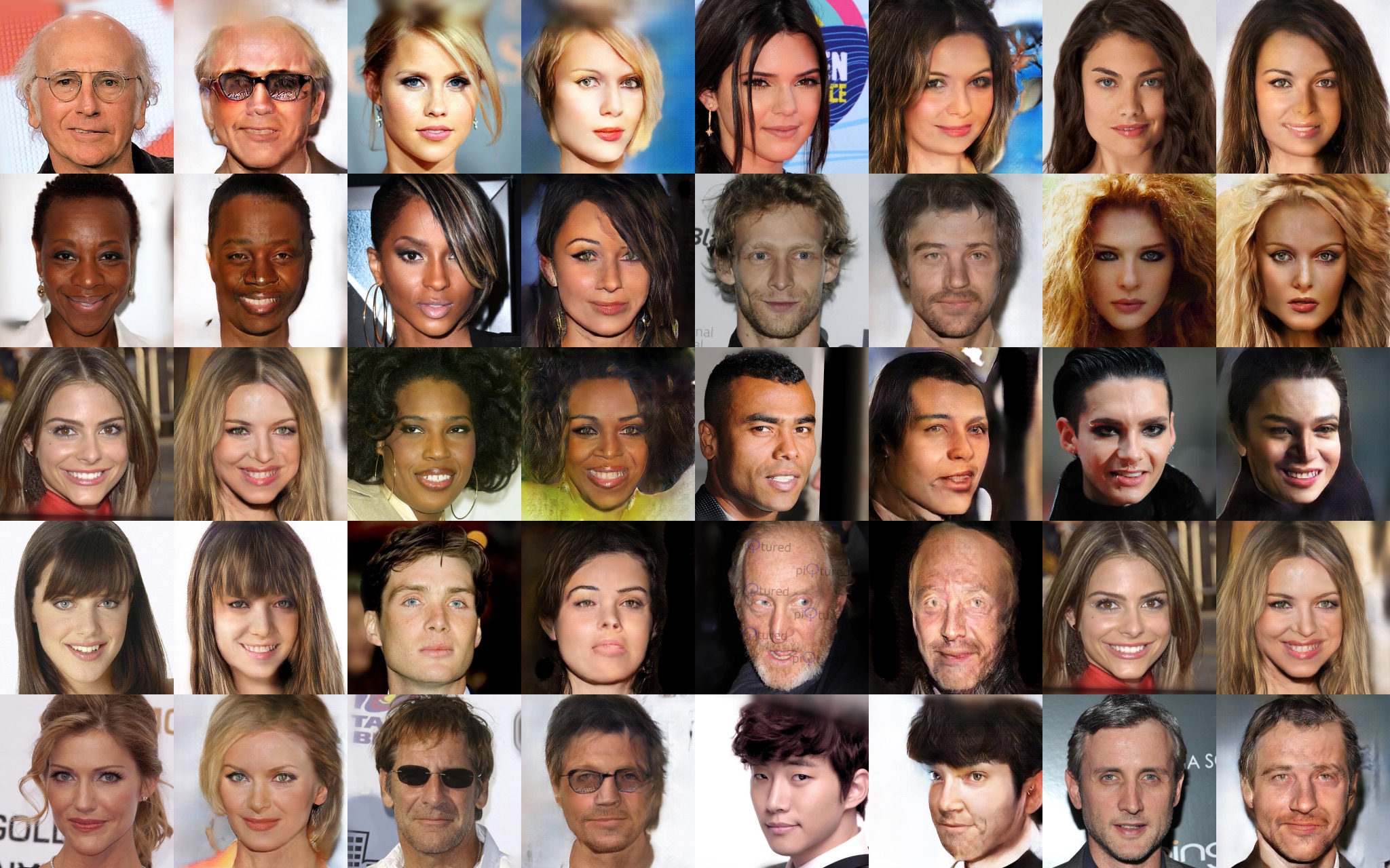
As we can see, both random generation and reconstruction yield satisfying results without blurriness. This indicates that we have successfully trained a GAN model that possesses both encoding and generation capabilities.
An important characteristic is that because this is dimensionality-reduction reconstruction, the model does not (and cannot) learn a pixel-by-pixel one-to-one mapping. Instead, it produces a clear reconstruction that looks "mostly the same" overall. For example, looking at the first image in the first row and the second image in the last row, the model basically reconstructs the person. Interestingly, regarding the glasses, we find that the model does reconstruct glasses but changes them to a different "style." We could even argue that the model has learned the concept of "glasses," but due to the limited expressive power of the latent variables in dimensionality reduction, it knows there are glasses but cannot reconstruct the exact same pair, so it substitutes them with a common style of glasses.
This is something that the "point-to-point reconstruction" required by standard VAEs cannot achieve; "point-to-point reconstruction" is also the main cause of blurriness in VAEs. If one requires perfectly reversible reconstruction, only reversible models like Glow are likely to achieve it.
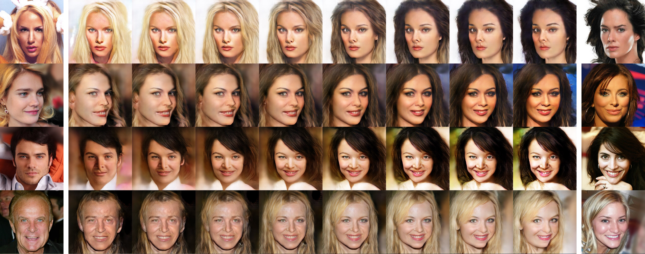
Additionally, since we have both an encoder and a generator, we can play with latent variable interpolation of real images:
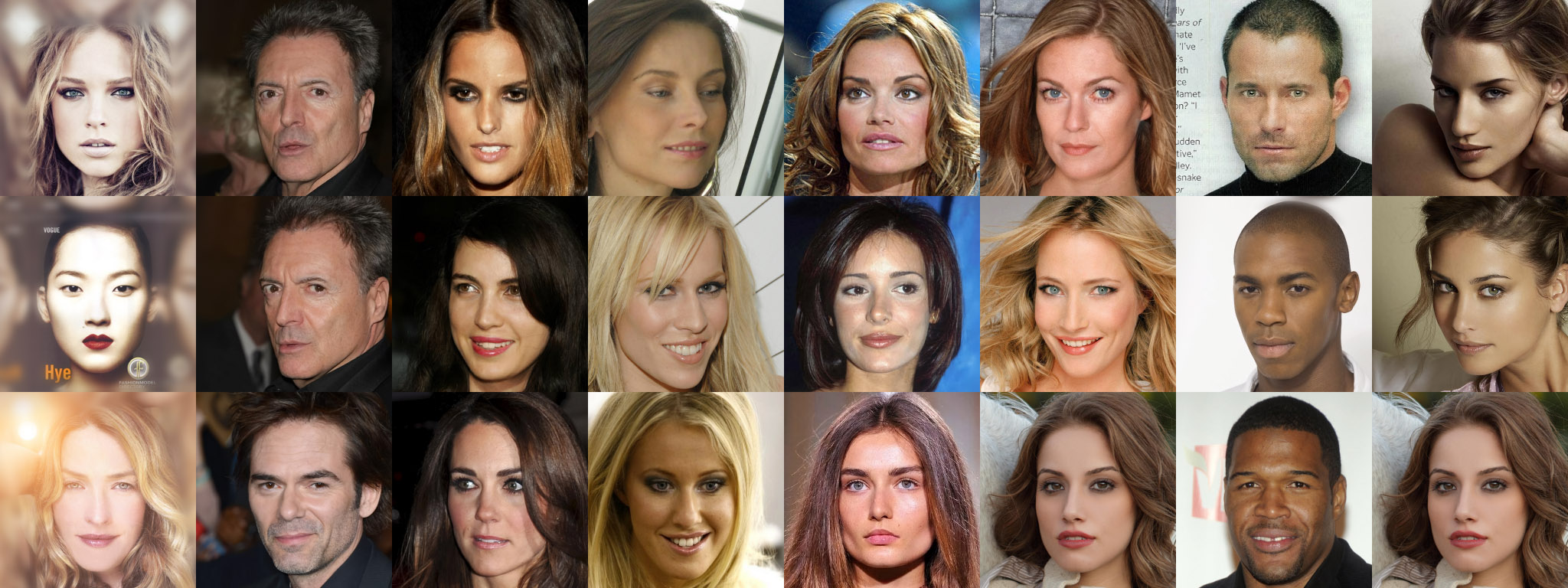
We can also look at similar images through the eyes of BiGAN-QP (calculate the latent variables for all real images, then use Euclidean distance or cosine similarity to find the most similar ones; the figure below shows results for Euclidean distance):