From the first article in this series to now, we have learned that the so-called “Minimum Entropy Principle” is dedicated to reducing learning costs, attempting to complete the same task with minimal effort. Therefore, this entire series is essentially a “Guide to Laziness.” So, what is the secret to being lazy? The answer is “routines” (patterns), which is why this series is also known as the “Collection of Routines.”
In this post, we will introduce the routines found in a library.
First, let’s pose a question: When did word vectors first appear? Was it Mikolov’s Word2Vec in 2013? Or Bengio’s neural language model in 2003? Neither. In fact, word vectors can be traced back thousands of years to ancient libraries...
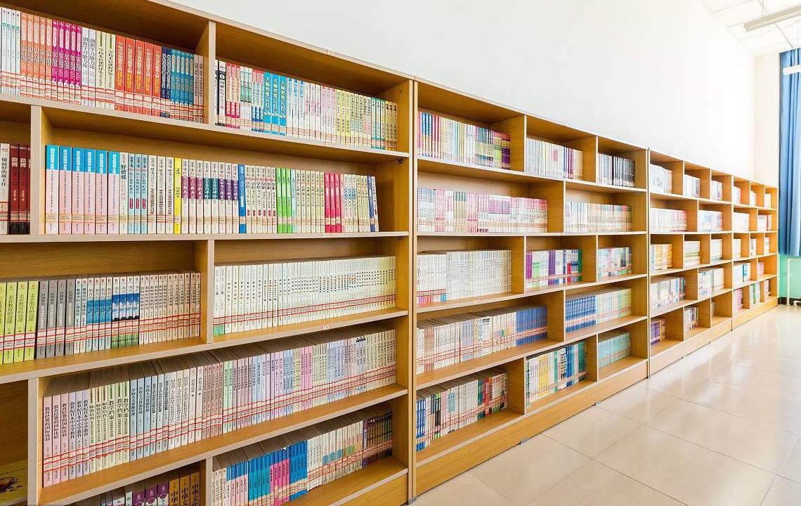
Walking into the Library
Word vectors in a library? Thousands of years ago? In which book? I’ll go borrow it and see.
The Routine of Placing Books
Actually, it’s not about a specific book, but the routine of how books are placed.
Obviously, the placement of books in a library follows a “routine”: they are not placed randomly but are categorized. For example, mathematics has one section, literature has another, and computer science has its own. Within the same category, there are many subcategories; for instance, in mathematics, mathematical analysis has a subsection, algebra has another, geometry has another, and so on. Have you ever wondered why they are categorized this way? What are the benefits of categorized placement? And what does it have to do with minimum entropy?
Some readers might think it’s simple: isn’t it just to make searching easier? This answer is actually not quite accurate. If it were only for the convenience of finding a book, it would be simple: just record the coordinates of every book in a database and mark the current coordinates on the floor. When you need to borrow a book, you check the coordinates in the database and go find it. This process doesn’t require “book classification” at all. Therefore, if we only consider the difficulty of finding a single book, we cannot explain this phenomenon well.
Borrowing Books Effortlessly
The core reason is: We usually don’t borrow just one book.
As mentioned, as long as an index is built, finding one book in a library is not difficult. The problem is: what if you want to find two? Generally, a person’s interests and research are relatively concentrated. Therefore, if I go to the library to borrow two books, it is reasonable to assume that the two books you want are related. For example, if you borrow a book on Neural Networks, the probability of borrowing another on Deep Learning is quite high, but the probability of borrowing Dream of the Red Chamber is very small. With the help of a database, I can quickly find Neural Networks. But what about Deep Learning? If this book is nearby, I only need to walk a few more steps to find it. If the books were placed randomly, I might have to walk from the southeast corner to the northwest corner to find Deep Learning. If I borrow a few more books, wouldn’t I have to run several laps around the library to collect them all?
In this way, the role of book classification becomes obvious. Book classification places similar books together, and the books a person borrows at one time are also likely to be similar. Therefore, book classification makes the process of finding and borrowing books more effortless for most people! This is another “Guide to Laziness.” In other words, organizing the things we process into categories and putting similar things together satisfies the Minimum Entropy Principle. In daily life, we categorize commonly used items and place them within reach based on the same principle.
Library Planning
Now let’s examine this process more closely from a mathematical perspective.
Simplified Borrowing Model
Suppose we go to the library to borrow two books, denoted as i and j. Assume the cost of finding the first book is d(i), and the cost function between the two books is d(i,j). This means that after finding the first book i, I have to spend d(i,j) amount of effort to find the second book j. We can consider the average of this process for everyone: S = \sum_{i,j} p(i)p(j|i) [d(i)+d(i,j)] = \sum_{i,j} p(i,j) [d(i)+d(i,j)] where p(i) is the probability of book i being borrowed, and p(j|i) is the probability that j will be borrowed after i is borrowed. To arrange books well, the library must minimize S.
Now, let’s take the library entrance as the origin and establish a three-dimensional coordinate system. The position of each book can be represented by a vector \boldsymbol{v}. Without loss of generality, we can simply consider d(i) as the Euclidean distance from the book to the library origin, and d(i,j) as the Euclidean distance between the two books. Then the expression for S becomes: S = \sum_{i,j} p(i,j) \left[\Vert \boldsymbol{v}_i\Vert + \Vert \boldsymbol{v}_i - \boldsymbol{v}_j\Vert\right] \label{eq:chengben}
Let’s explain the meaning of each term again. Here, (i,j) represents a borrowing habit (borrowing book i and then book j), and p(i,j) represents the probability of this habit occurring, which can be estimated from library borrowing records in real life. \Vert \boldsymbol{v}_i\Vert + \Vert \boldsymbol{v}_i - \boldsymbol{v}_j\Vert represents the total cost of borrowing i and then j. Minimizing \Vert \boldsymbol{v}_i\Vert means we should place popular books near the exit (origin), while minimizing \Vert \boldsymbol{v}_i - \boldsymbol{v}_j\Vert tells us to put similar books together.
Constrained Optimization Planning
If we have the library’s borrowing records, meaning p(i,j) is known, can we obtain the “optimal book arrangement” by minimizing Eq. [eq:chengben]? The idea is correct, but incomplete, because the minimum value of Eq. [eq:chengben] is obviously 0, which would require all \boldsymbol{v} to be 0—meaning all books are crammed at the exit.
Obviously, this is impossible because books are not infinitely small; there is a minimum distance d_{\min} > 0 between two books. So the complete formulation should be: \begin{aligned}S =& \min_{\boldsymbol{v}}\sum_{i,j} p(i,j) \left[\Vert \boldsymbol{v}_i\Vert + \Vert \boldsymbol{v}_i - \boldsymbol{v}_j\Vert\right] \\ &\text{s.t.}\quad\forall i\neq j,\, \Vert \boldsymbol{v}_i - \boldsymbol{v}_j\Vert \geq d_{\min} \end{aligned}\label{eq:chengben-2} In other words, this is a constrained optimization problem. Solving this problem gives us the most reasonable arrangement of books for the library (theoretically). Of course, if we were actually planning a library, we would introduce more constraints based on the actual situation, such as the shape of the library and the layout of the aisles, but Eq. [eq:chengben-2] is sufficient for us to understand the fundamental idea.
General Cost Minimization
Now let’s generalize the problem and observe it from a more abstract perspective to gain deeper insights.
Uniformity and De-constraining
We first replace the cost function \Vert \boldsymbol{v}_i\Vert + \Vert \boldsymbol{v}_i - \boldsymbol{v}_j\Vert with a general f(\boldsymbol{v}_i,\boldsymbol{v}_j), considering: S = \sum_{i,j} p(i,j) f(\boldsymbol{v}_i,\boldsymbol{v}_j)\label{eq:yibanchengben} Meanwhile, \boldsymbol{v} is no longer limited to a 3D vector but can be a general n-dimensional vector. We still want to minimize the cost, but we dislike constraints like \Vert \boldsymbol{v}_i - \boldsymbol{v}_j\Vert \geq d_{\min} because constrained optimization problems are often difficult to solve. If we can reflect this constraint directly in the choice of f, it would be an elegant “de-constraining” solution.
How do we achieve this? Returning to the library problem, without constraints, the theoretical optimal solution is to cram all books at the exit. To prevent this unreasonable solution, we added the constraint “a minimum distance d_{\min} > 0 between two books” to prevent the collapse of the solution. In fact, many other constraints can be considered; for example, we can require all books to be spread as uniformly as possible throughout the library. Under this expectation, a reasonable solution can also be obtained.
“Uniformity” can be understood as a kind of normalization constraint. Because of normalization, they cannot all be concentrated at one point, as a single point is not normalized. “Normalization” inspires us to think in the direction of probability—that is, first construct a probability distribution and then use it as a measure of the cost function. Without too much forced guidance, I will directly give one choice: f(\boldsymbol{v}_i,\boldsymbol{v}_j)=-\log\frac{e^{-\left\Vert\boldsymbol{v}_i-\boldsymbol{v}_j\right\Vert^2}}{Z_i},\quad Z_i = \sum_j e^{-\left\Vert\boldsymbol{v}_i-\boldsymbol{v}_j\right\Vert^2}\label{eq:chengben-l2}
Minimum Entropy = Maximum Likelihood
Let’s understand this formula step by step. First, if we ignore the denominator Z_i, the result is: -\log \left(e^{-\left\Vert\boldsymbol{v}_i-\boldsymbol{v}_j\right\Vert^2}\right) =\left\Vert\boldsymbol{v}_i-\boldsymbol{v}_j\right\Vert^2 That is, this f is equivalent to a cost function of \left\Vert\boldsymbol{v}_i-\boldsymbol{v}_j\right\Vert^2. Then, because of the denominator, we know: \sum_j\frac{e^{-\left\Vert\boldsymbol{v}_i-\boldsymbol{v}_j\right\Vert^2}}{Z_i}=1 So e^{-\left\Vert\boldsymbol{v}_i-\boldsymbol{v}_j\right\Vert^2}/Z_i actually defines a conditional probability distribution q(j|i). Simply put, this is a softmax operation on -\left\Vert\boldsymbol{v}_i-\boldsymbol{v}_j\right\Vert^2, and at this point, Eq. [eq:yibanchengben] is actually: S = -\sum_{i,j} p(i)p(j|i) \log q(j|i)\label{eq:gailvchengben} For a fixed i, minimizing the above expression is equivalent to maximum log-likelihood! Therefore, the result is that q(j|i) will try to be as close to p(j|i) as possible. Thus, taking all values as 0 is not necessarily the optimal solution, because all 0s correspond to a uniform distribution, while the true p(j|i) is not necessarily uniform.
Now think about it: starting from the idea of minimum cost, we designed an f(\boldsymbol{v}_i,\boldsymbol{v}_j) in the form of a negative log-probability, and found that the final result is maximum likelihood. This result is both unexpected and reasonable, because the meaning of -\log q(j|i) is entropy. We say we want maximum likelihood, which means minimizing Eq. [eq:gailvchengben], the meaning of which is minimum entropy. Maximum likelihood and minimum entropy actually share the same meaning.
Word2Vec
By slightly changing the object, Word2Vec emerges, or even everything2vec...
Diverse Metrics
From a purely formal perspective, although the choice in Eq. [eq:chengben-l2] is intuitive, it is not the only one. Another viable choice is: f(\boldsymbol{v}_i,\boldsymbol{v}_j)=-\log\frac{e^{\left\langle\boldsymbol{v}_i,\boldsymbol{v}_j\right\rangle}}{Z_i},\quad Z_i = \sum_j e^{\left\langle\boldsymbol{v}_i,\boldsymbol{v}_j\right\rangle}\label{eq:chengben-dot} This uses the dot product as a distance metric, hoping that the dot product of similar objects is as large as possible (so the negative log is small).
Skip-Gram
In fact, if i and j represent words within a sentence window, then Eq. [eq:chengben-dot] corresponds to the famous word vector model—the Skip-Gram model of Word2Vec. That is, minimizing: S = -\sum_{i,j} p(i,j) \log\frac{e^{\left\langle\boldsymbol{v}_i,\boldsymbol{v}_j\right\rangle}}{Z_i}\label{eq:word2vec} This is exactly the optimization objective of the Word2Vec Skip-Gram model.
Note: Word2Vec actually distinguishes between context vectors and center word vectors, using two sets of word vectors. However, to intuitively understand the underlying idea, we do not make that distinction here.
Analogical Analysis of Principles
Wait, how did word vectors suddenly appear?
Let’s retrace our logic: We treat each word as a book, and each sentence can be seen as a person’s “borrowing record.” This way, we can know which two “books” are often borrowed together. According to the optimal library book arrangement scheme we discussed, we can find the optimal positions for the “books.” Theoretically, using Eq. [eq:chengben-2], [eq:chengben-l2], or [eq:chengben-dot] works; these are word vectors! If we use Eq. [eq:chengben-dot], it is Word2Vec.
Conversely, finding an optimal book arrangement scheme becomes simple: treat every person’s borrowing record in the library as a sentence, each book as a word, set the word vector dimension to 3, and train it with Word2Vec. The resulting word vectors are the optimal book arrangement.
Methods like doc2vec, node2vec, and everything2vec are basically done this way.
So, the initial question becomes clear: Recording the 3D coordinates of every book in a library is a literal “book embedding.” The vectors of similar books are also similar, perfectly corresponding to the characteristics of word vectors. Thus, since libraries existed, embeddings have existed, even though there were no coordinate systems or computers back then.
A Look at t-SNE
With “borrowing records,” i.e., p(j|i) and p(i), we can follow the above process to get an “optimal position plan,” which is the process of vectorization.
What if we don’t have them?
SNE
Then create them! For example, if we have a set of high-dimensional samples \boldsymbol{x}_1, \boldsymbol{x}_2, \dots, \boldsymbol{x}_N (e.g., an image dataset) and we want to obtain a low-dimensional representation \boldsymbol{z}_1, \boldsymbol{z}_2, \dots, \boldsymbol{z}_N. We construct: p(\boldsymbol{x}_j|\boldsymbol{x}_i)=\frac{e^{-\Vert \boldsymbol{x}_i-\boldsymbol{x}_j\Vert^2/2\sigma^2}}{\sum\limits_{j}^{j\neq i}e^{-\Vert \boldsymbol{x}_i-\boldsymbol{x}_j\Vert^2/2\sigma^2}}\label{eq:pij} Then we still use Eq. [eq:chengben-l2] as the cost function (assuming p(i) is a constant, i.e., a uniform distribution, and the summation excludes the self-term) to optimize Eq. [eq:yibanchengben]: S=-\sum_{i,j}^{i\neq j}p(\boldsymbol{x}_j|\boldsymbol{x}_i)\log q(j|i),\quad q(j|i)=\frac{e^{-\left\Vert\boldsymbol{z}_i-\boldsymbol{z}_j\right\Vert^2}}{\sum\limits_{j}^{j\neq i}e^{-\left\Vert\boldsymbol{z}_i-\boldsymbol{z}_j\right\Vert^2}} This is the dimensionality reduction method known as SNE (Stochastic Neighbor Embedding).
Generally, there are some variants, but we won’t go into details as they are not the focus of this article. We only need to understand the basic idea. SNE is essentially a dimensionality reduction scheme that tries to maintain relative distances. Because it maintains relative distances, it preserves the basic shape, making its dimensionality reduction effect better than methods like PCA. The reason is that PCA only retains principal components and is only suitable for relatively regular data (e.g., those with central clustering and isotropy). The idea of SNE can be applied to any connected shape.
t-SNE
The SNE mentioned above already embodies the idea of dimensionality reduction. However, it has some problems, primarily the “Crowding Problem.” Simply put, the Crowding Problem occurs because the low-dimensional distribution in Eq. [eq:chengben-l2] is also in the form of a negative exponential of distance. The problem with a negative exponential is that it decays rapidly to 0 at a distance. Since \boldsymbol{z} in Eq. [eq:chengben-l2] is our optimization target, the result is that almost all points crowd together near some location (because of the exponential decay, distant points almost never appear), leading to poor results.
To solve this problem, we can replace Eq. [eq:chengben-l2] with a function that decays more slowly, such as a simple fraction: f(\boldsymbol{z}_i,\boldsymbol{z}_j)=-\log\frac{(1+\left\Vert\boldsymbol{z}_i-\boldsymbol{z}_j\right\Vert^2)^{-1}}{Z_i},\quad Z_i = \sum_{j}^{j\neq i} (1+\left\Vert\boldsymbol{z}_i-\boldsymbol{z}_j\right\Vert^2)^{-1}\label{eq:t} This is known as the t-distribution. Combining Eq. [eq:t], Eq. [eq:pij], and Eq. [eq:yibanchengben] results in the dimensionality reduction method called t-SNE. Compared to SNE, it improves the Crowding Problem.
Of course, the difference between t-SNE and SNE is not the focus of this article. The focus is to reveal the similarities between dimensionality reduction algorithms like SNE and Word2Vec.
Although in deep learning we don’t often use dimensionality reduction methods like t-SNE directly—since there are many more elegant schemes for dimensionality reduction and clustering (for dimensionality reduction, see “Mutual Information in Deep Learning: Unsupervised Feature Extraction”; for clustering, see “Variational Autoencoders (IV): A One-Step Clustering Solution”)—the essential idea of t-SNE is reflected in many scenarios. Therefore, digging into and savoring its principles and connecting them with other knowledge points to form one’s own knowledge system is a worthwhile endeavor.
Summary
Based on the idea of minimum cost, this article constructed an idealized model to analyze the principles of book arrangement in a library, linked it to the Minimum Entropy Principle, and reflected on its connections with Word2Vec and t-SNE. Thus, we have formed more vivid examples of the Minimum Entropy Principle: Birds of a feather flock together, and categorization reduces costs. For example, we can now understand why pre-trained word vectors can speed up the convergence of NLP tasks and sometimes improve final results: because word vectors place words in suitable positions in advance, and their construction principle itself is to reduce costs.
At the same time, connecting many seemingly unrelated things can promote mutual understanding and achieve the effect of comprehensive mastery, the beauty of which is beyond words.
Original Address: https://kexue.fm/archives/6191
For more details on reprinting, please refer to: “Scientific Space FAQ”