From Variational Encoding and Information Bottleneck to Normal Distribution: On the Importance of Forgetting

Theoretical Review

Briefly, the optimization objective of a VAE is: KL(\tilde{p}(x)p(z|x)\Vert q(z)q(x|z))=\iint \tilde{p}(x)p(z|x)\log \frac{\tilde{p}(x)p(z|x)}{q(x|z)q(z)} dzdx where q(z) is the standard normal distribution, and p(z|x), q(x|z) are conditional normal distributions corresponding to the encoder and decoder, respectively. For specific details, please refer to "Variational Autoencoder (II): A Bayesian Perspective".

This objective can ultimately be simplified to: \mathbb{E}_{x\sim \tilde{p}(x)} \Big[\mathbb{E}_{z\sim p(z|x)}\big[-\log q(x|z)\big]+KL\big(p(z|x)\big\Vert q(z)\big)\Big] \label{eq:vae} Clearly, it can be viewed in two parts: the term \mathbb{E}_{z\sim p(z|x)}\big[-\log q(x|z)\big] is equivalent to a standard autoencoder loss (with the reparameterization trick), and KL\big(p(z|x)\big\Vert q(z)\big) is the KL divergence between the posterior and the prior. The first term aims to minimize reconstruction loss, meaning it wants the latent variable z to retain as much information as possible. The second term aligns the latent space with a normal distribution, meaning it wants the distribution of latent variables to be more regular.

Comparison with Autoencoders

Compared to a standard autoencoder, the changes in a VAE are:

1. It introduces the concepts of mean and variance and incorporates the reparameterization trick.

2. It adds KL divergence as an additional loss function.

Unveiling the Black Box of Deep Learning?

In September last year, there was a presentation on Deep Learning and the Information Bottleneck which claimed to unveil the "black box" of Deep Learning (DL). After hearing it, the great Geoffrey Hinton commented, "This is so interesting, I need to watch it another 10,000 times..." (refer to "Unveiling the Black Box of Deep Learning: Hebrew University Professor Proposes Information Bottleneck"). Consequently, the Information Bottleneck became a hot topic. Shortly thereafter, an article challenged these results, suggesting that the conclusions of the Information Bottleneck are not universal (refer to "Bursting the Bubble: A Critical Analysis of the Information Bottleneck Theory"), making the discussion even more lively.

Regardless of whether the Information Bottleneck can reveal the secrets of deep learning, as practitioners, we primarily look at whether it can extract something valuable for use. The so-called Information Bottleneck is a simple idea: it says that when faced with a task, a model attempts to complete it using the minimum amount of information. This is similar to our previous discussion on the "Minimum Entropy Series", because information corresponds to learning cost. Completing a task with minimal information means completing it at the lowest cost, which implies obtaining a model with better generalization performance.

Principles of Information Bottleneck

Why does lower cost/less information lead to better generalization? This is not hard to understand. For example, in a company, if we were to customize a solution for every single client and assign dedicated personnel to follow up, the cost would be enormous. If we can find a universal solution and only perform fine-tuning on that basis, the cost becomes much lower. A "universal solution" exists because we have found the commonalities and patterns in client needs. Thus, a minimum-cost solution implies that we have found universal laws and characteristics, which translates to generalization performance.

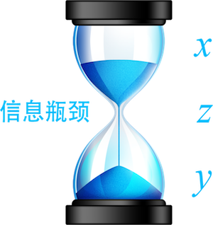
How do we reflect this in deep learning? The answer is the Variational Information Bottleneck (VIB), originating from the paper "Deep Variational Information Bottleneck".

Suppose we are facing a classification task with labeled data pairs (x_1, y_1), \dots, (x_N, y_N). We can understand this task in two steps: the first is encoding, and the second is classification. The first step encodes x into a latent variable z, and then the classifier identifies z as category y: x \quad \to \quad z \quad \to \quad y

Now imagine adding a "bottleneck" \beta at z. It acts like an hourglass; the amount of incoming information might be large, but the exit is only as wide as \beta. Thus, the role of this bottleneck is to prevent the amount of information flowing through z from exceeding \beta. Unlike an hourglass where sand just passes through, information passing through the bottleneck must still complete its task (classification, regression, etc.). Therefore, the model is forced to find a way to let only the most important information pass through. This is the principle of the Information Bottleneck.

Variational Information Bottleneck

How is this operated quantitatively? We use "Mutual Information" as the metric to measure the amount of information passed: \iint p(z|x)\tilde{p}(x)\log \frac{p(z|x)}{p(z)}dxdz Here p(z) is not an arbitrarily specified distribution, but the true distribution of the latent variables. Theoretically, after knowing p(z|x), we can calculate p(z), as it is formally equal to: p(z) = \int p(z|x)\tilde{p}(x)dx Of course, this integral is often difficult to compute, so we will look for another way.

Additionally, we have the task loss, such as cross-entropy for classification: -\iint p(z|x)\tilde{p}(x)\log p(y|z)dxdz Writing it in this form indicates we have an encoder that first encodes x into z, and then classifies z.

How do we "prevent the information flowing through z from exceeding \beta"? We can add it directly as a penalty term, making the final loss: -\iint p(z|x)\tilde{p}(x)\log p(y|z)dxdz + \lambda \iint p(z|x)\tilde{p}(x)\max\left(\log \frac{p(z|x)}{p(z)} - \beta, 0\right)dxdz That is, once the mutual information exceeds \beta, a positive penalty term appears. Often, we don’t know what value to set for \beta, so a more straightforward approach is to remove \beta, yielding: -\iint p(z|x)\tilde{p}(x)\log p(y|z)dxdz + \lambda \iint p(z|x)\tilde{p}(x)\log \frac{p(z|x)}{p(z)}dxdz This simply encourages the amount of information to be as small as possible without setting a specific threshold.

Now we have the formula, but as we said, p(z) is uncalculable. We must estimate its upper bound: assuming q(z) is a distribution with a known form, we have: \begin{aligned} &\iint p(z|x)\tilde{p}(x)\log \frac{p(z|x)}{p(z)}dxdz\\ =& \iint p(z|x)\tilde{p}(x)\log \frac{p(z|x)}{q(z)}\frac{q(z)}{p(z)}dxdz\\ =& \iint p(z|x)\tilde{p}(x)\log \frac{p(z|x)}{q(z)} + \iint p(z|x)\tilde{p}(x)\log \frac{q(z)}{p(z)}dxdz\\ =& \iint p(z|x)\tilde{p}(x)\log \frac{p(z|x)}{q(z)} + \int p(z)\log \frac{q(z)}{p(z)}dz\\ =& \iint p(z|x)\tilde{p}(x)\log \frac{p(z|x)}{q(z)} - \int p(z)\log \frac{p(z)}{q(z)}dz\\ =& \int \tilde{p}(x) KL\big(p(z|x)\big\Vert q(z)\big) dx - KL\big(p(z)\big\Vert q(z)\big)\\ <& \int \tilde{p}(x) KL\big(p(z|x)\big\Vert q(z)\big) dx \end{aligned} This shows that \int\tilde{p}(x) KL\big(p(z|x)\big\Vert q(z)\big) dx is an upper bound for the mutual information. If we optimize the former, the latter will not exceed it. Since the latter cannot be calculated directly, we optimize the former. Thus, the final usable loss is: -\iint p(z|x)\tilde{p}(x)\log p(y|z)dxdz + \lambda \int\tilde{p}(x) KL\big(p(z|x)\big\Vert q(z)\big) dx Or equivalently: \mathbb{E}_{x\sim \tilde{p}(x)} \Big[\mathbb{E}_{z\sim p(z|x)}\big[-\log p(y|z)\big]+\lambda\cdot KL\big(p(z|x)\big\Vert q(z)\big)\Big] \label{eq:vib} This is the Variational Information Bottleneck.

Observations and Implementation

It can be seen that if q(z) is taken as the standard normal distribution (which we almost always do), Equation [eq:vib] is nearly identical to the VAE loss function [eq:vae]. The difference is that [eq:vib] discusses supervised tasks, while [eq:vae] is for unsupervised learning. However, if we view VAE as a supervised task where the label is the input x itself, then it is a special case of [eq:vib].

So, compared to the original supervised learning task, the changes in the Variational Information Bottleneck are:

1. It introduces the concepts of mean and variance and incorporates the reparameterization trick.

2. It adds KL divergence as an additional loss function.

Exactly like VAE!

Implementing VIB in Keras is very simple. I have defined a layer for easy use:

from keras.layers import Layer
import keras.backend as K

class VIB(Layer):
    """Variational Information Bottleneck Layer
    """
    def __init__(self, lamb, **kwargs):
        self.lamb = lamb
        super(VIB, self).__init__(**kwargs)
        
    def call(self, inputs):
        z_mean, z_log_var = inputs
        u = K.random_normal(shape=K.shape(z_mean))
        kl_loss = - 0.5 * K.sum(K.mean(1 + z_log_var - K.square(z_mean) - K.exp(z_log_var), 0))
        self.add_loss(self.lamb * kl_loss)
        u = K.in_train_phase(u, 0.)
        return z_mean + K.exp(z_log_var / 2) * u
        
    def compute_output_shape(self, input_shape):
        return input_shape[0]

The usage is simple, requiring only minor changes to the original task. Please refer to: https://github.com/bojone/vib/blob/master/cnn_imdb_vib.py

Effect: Compared to models without VIB, models with VIB converge faster and easily reach over 89% validation accuracy, whereas models without VIB usually only reach around 88% and converge more slowly.

Variational Discriminator Bottleneck

The original paper "Deep Variational Information Bottleneck" showed that VIB is a quite effective regularization method, improving performance across multiple tasks.

However, the story of the Information Bottleneck doesn’t end there. Not long ago, a paper titled "Variational Discriminator Bottleneck" was rated as a high-score paper for ICLR 2019 (appearing alongside the famous BigGAN). The authors were no longer satisfied with applying VIB only to standard supervised tasks; the paper developed the "Variational Discriminator Bottleneck" and applied it to GANs, reinforcement learning, and other tasks, achieving improvements in all of them! The power of the Information Bottleneck is evident.

Unlike Equation [eq:vib], the "Variational Discriminator Bottleneck" paper modified the update mechanism to give it some adaptive capability, but the fundamental idea remains the same: regularizing the model by limiting mutual information. However, this is no longer the focus of this article; interested readers should refer to the original paper.

Regularization and Decoupling

In fact, one could write an entire book about the origins, stories, and uses of the normal distribution. Many properties of the normal distribution have been discussed elsewhere; here, I will only introduce the parts relevant to this article.

The role of KL divergence is to align the latent variable distribution with a (multivariate) standard normal distribution, rather than any arbitrary normal distribution. The standard normal distribution is relatively regular, with benefits like zero mean and unit variance. More importantly, the standard normal distribution has a very valuable characteristic: its components are decoupled. In probabilistic terms, they are independent, satisfying p(x,y)=p(x)p(y).

We know that if features are independent, modeling becomes much easier (a Naive Bayes classifier would be a perfectly accurate model), and independent features are much more interpretable. Therefore, we always hope for independent features. As early as 1992, the father of LSTM, Schmidhuber, proposed the PM model (Predictability Minimization), dedicated to building an autoencoder with decoupled features. You can refer to the related story "From PM to GAN - LSTM Father Schmidhuber’s 22-Year Grudge". Yes, in the years before I even arrived on Earth, the giants were already researching feature decoupling, showing how valuable it is.

In VAEs (including later Adversarial Autoencoders), the KL divergence directly aligns the latent variable distribution with a decoupled prior. The benefit is that the latent variables themselves become nearly decoupled, thus possessing the various advantages mentioned above. Therefore, we can now answer a question that is likely to be asked:

Q: From the perspective of feature encoding, what are the advantages of a Variational Autoencoder compared to a standard autoencoder?

A: The VAE uses KL divergence to bring the latent variable distribution closer to a standard normal distribution, thereby decoupling latent features and simplifying subsequent models built on those features. (Of course, you can also answer by mentioning the Variational Information Bottleneck discussed earlier, such as enhancing generalization performance, etc. ^_^)

Linear Interpolation and Convolution

Furthermore, the normal distribution has another important property, which is often used to demonstrate the effects of generative models: linear interpolation.

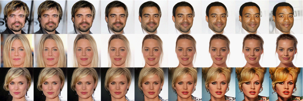
The process of this linear interpolation is: first sample two random vectors z_1, z_2 \sim \mathcal{N}(0, 1). Clearly, a good generator can turn z_1, z_2 into realistic images g(z_1), g(z_2). Then we consider g(z_{\alpha}), where: z_{\alpha} = (1 - \alpha) z_1 + \alpha z_2, \quad 0 \leq \alpha \leq 1 As \alpha changes from 0 to 1, we expect to see g(z_{\alpha}) as a gradual transition from image g(z_1) to image g(z_2), and indeed this is the case.

Why must interpolation happen in the latent space? Why does interpolating directly between original images not yield meaningful results? This is actually related to the normal distribution, because we have the following convolution theorem (this "convolution" is the mathematical operator, not the convolutional layer in a neural network):

If z_1 \sim \mathcal{N}(\mu_1, \sigma_1^2) and z_2 \sim \mathcal{N}(\mu_2, \sigma_2^2) are independent random variables, then: z_1 + z_2 \sim \mathcal{N}(\mu_1+\mu_2, \sigma_1^2+\sigma_2^2) Specifically, if z_1 \sim \mathcal{N}(0, 1) and z_2 \sim \mathcal{N}(0, 1), then: \alpha z_1 + \beta z_2 \sim \mathcal{N}(0, \alpha^2+\beta^2)

This means that the sum of normal random variables is still a normal random variable. What does this imply? It means that in the world of normal distributions, the linear interpolation of two variables still resides within that world. This is not a common property, as interpolating between two real samples does not necessarily result in a realistic image.

For supervised tasks, what is the value of this linear interpolation property? It is very important. We know that labeled datasets are hard to come by. If we can reasonably map the latent space of a finite training set to a standard normal distribution, then we can expect that parts not covered by the training set might also be considered, because their latent variables might just be linear interpolations of the original training set’s latent variables.

In other words, when we complete supervised training and regularize the latent distribution to a standard normal distribution, we have effectively included the transition samples between training instances, which is equivalent to covering more samples.

Note: We usually consider uniform linear interpolation in the spatial domain, i.e., the form \beta = 1-\alpha. However, from the perspective of \alpha z_1 + \beta z_2 \sim \mathcal{N}(0, \alpha^2+\beta^2), the best choice is interpolation where \alpha^2+\beta^2=1, namely: z_{\theta}=z_1\cdot\cos\theta + z_2\cdot\sin\theta Secondly, readers might wonder: when the prior distribution of a GAN is a uniform distribution, can’t we also perform linear interpolation? This doesn’t seem unique to the normal distribution. In fact, the convolution of uniform distributions is no longer a uniform distribution, but its probability density function happens to concentrate in the middle of the original uniform distribution (though it is no longer uniform, it’s like taking a subset of the original), so the interpolation effect is still satisfactory. However, theoretically, it is not as elegant. Furthermore, in practice, normal distributions are now mostly used in GAN training, as they perform better than uniform distributions.