I don’t know when it started, but I found myself falling into the deep pit of GANs. Sigh, I hope I can jump out of it soon...
This blog post introduces a new GAN framework I recently submitted to arXiv. It primarily presents a new understanding of probability divergence and derives a new GAN based on this understanding. The entire article is quite theoretical, with complete proofs for the relevant properties of this GAN. I consider it a theoretically sound result.
Paper link: https://papers.cool/arxiv/1811.07296
First, the conclusions:
The paper provides a direct approach for analyzing and constructing probability divergences, thereby simplifying the process of building new GAN frameworks.
It derives a GAN framework called GAN-QP [eq:gan-gp-gd]. This GAN does not require Lipschitz (L) constraints like WGAN, nor does it suffer from the vanishing gradient problem of SGAN. Experiments show that its performance is at least comparable to, if not better than, WGAN.
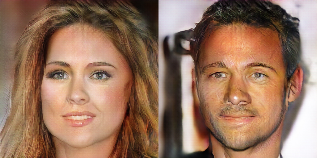
The experiments in the paper reached up to 512 \times 512 face generation (CelebA HQ), fully demonstrating the effectiveness of the model (the results are not perfect, but the model is exceptionally simple). Interested friends, please read on.
Facing the Dual Space
To construct a GAN framework, we generally follow three steps:
Seek a good probability divergence;
Find its dual form;
Transform it into a min-max game.
The problem is: what is truly useful for the training process are the second and third steps; the first step is not strictly necessary.
In fact, it is difficult to define a new divergence from the primal space, and even if defined, it might not be easy to transform into a dual form. However, we can analyze directly in the dual space, which allows us to discover a batch of new, well-behaved divergences. In other words, we can directly argue whether an expression satisfies the definition of a divergence in the dual space, thereby directly providing an optimizable objective without needing to care whether it is specifically JS divergence or Wasserstein distance.
Let’s illustrate this idea with examples.
Divergence
First, let’s give the definition of a divergence:
If \mathcal{D}[p, q] is a scalar function of p and q that satisfies:
\mathcal{D}[p, q] \geq 0 always holds;
\mathcal{D}[p, q] = 0 \Leftrightarrow p = q.
Then \mathcal{D}[p, q] is called a divergence between p and q. The main difference between a divergence and a "distance" is that a divergence does not need to satisfy the triangle inequality or symmetry. However, a divergence retains the most basic properties for measuring gaps, so we can use it to measure the degree of difference between p and q.
SGAN
Basic Definition
Let’s first look at the discriminator loss in SGAN, defined as: \mathcal{D}[p(x), q(x)] = \max_T \frac{1}{2}\mathbb{E}_{x \sim p(x)}[\log \sigma(T(x))] + \frac{1}{2}\mathbb{E}_{x \sim q(x)}[\log (1 - \sigma(T(x)))] + \log 2 \label{eq:js-dual-2} This is actually the dual form of the JS divergence. However, we can prove it is a divergence directly based on this definition and discuss its properties without even knowing it is the JS divergence.
How to prove it? We only need to prove that this result satisfies the two requirements of a divergence mentioned above. Note that according to our logic, we don’t know it’s JS divergence, but we can prove it’s a divergence from a mathematical perspective.
If the reader truly understands the meaning of Equation [eq:js-dual-2], the proof is not difficult. Equation [eq:js-dual-2] first defines an expectation formula and then takes the maximum over T (more accurately, the "supremum"). Only the result of taking the maximum is the divergence. To emphasize again: "the result after taking the maximum is the divergence"; the expression \frac{1}{2}\mathbb{E}_{x \sim p(x)}[\log \sigma(T(x))] + \frac{1}{2}\mathbb{E}_{x \sim q(x)}[\log (1 - \sigma(T(x)))] + \log 2 itself is not a divergence.
The specific proof process is somewhat lengthy and won’t be fully presented here; please refer to the appendix of the original paper. Alternatively, look at the WGAN section below, as it is relatively simpler.
Adversarial Networks
Once we have a divergence, we can train a generative model by minimizing the divergence between two probability distributions. That is, the next step is: \min_{G} \mathcal{D}[p(x), q(x)] Note that \mathcal{D}[p(x), q(x)] is achieved through the \max_T operation, so the combination is a min-max process. For the previous example, this is equivalent to: G, T = \mathop{\text{argmin}}_G \mathop{\text{argmax}}_T \mathbb{E}_{x \sim p(x)}[\log \sigma(T(x))] + \mathbb{E}_{x=G(z), z \sim q(z)}[\log (1 - \sigma(T(x)))] \label{eq:js-min-max} This is SGAN.
So we find that the GAN process actually consists of two steps: 1. Define a divergence through \max; 2. Minimize the divergence between two distributions through \min. The new perspective here is to treat \max directly as part of the definition of the divergence.
Performance Analysis
We know that SGAN may suffer from the risk of vanishing gradients. Why is this? Let’s examine an extreme case: p(x) = \delta(x - \alpha), \quad q(x) = \delta(x - \beta) where \alpha \neq \beta. In this case, the two distributions are just single-point distributions with no overlap. Substituting this into [eq:js-dual-2], the result is: \mathcal{D}[p(x), q(x)] = \max_T \frac{1}{2}[\log \sigma(T(\alpha))] + \frac{1}{2}[\log (1 - \sigma(T(\beta)))] + \log 2 Since we have no constraints on T, to maximize this, we can let T(\alpha) \to +\infty and T(\beta) \to -\infty, resulting in a supremum that is the constant \log 2. That is, in this case, \mathcal{D}[p(x), q(x)] = \log 2.
This means that for two distributions with almost no overlap, the divergence defined by Equation [eq:js-dual-2] yields a constant \log 2. A constant means the gradient is 0, making optimization impossible. The two WGAN papers showed that "no overlap" is theoretically very common in GANs, so this is an inherent flaw of SGAN.
General f-divergences
The previous subsections have fully presented the workflow of this understanding:
We define a mathematical expression through \max, and then prove from a mathematical perspective that it is a divergence, without caring what it is called;
We minimize this divergence through \min, and the combination is a min-max process, resulting in a type of GAN;
To check the performance of this divergence in extreme cases, we can test it with p(x) = \delta(x - \alpha), q(x) = \delta(x - \beta).
The above discussion regarding SGAN can be extended in parallel to all f-GANs. Various f-divergences are not essentially different; they share the same inherent flaws (either vanishing gradients or exploding gradients).
WGAN
Basic Definition
Now we turn to a new class of divergence: Wasserstein distance. Note that Wasserstein distance is a strict distance satisfying axiomatic definitions, but here we only care about its divergence properties. Define: \mathcal{W}[p(x), q(x)] = \max_{T, \|T\|_L \leq 1} \mathbb{E}_{x \sim p(x)}[T(x)] - \mathbb{E}_{x \sim q(x)}[T(x)] \label{eq:wd-dual} where \|T\|_L = \max_{x \neq y} \frac{|T(x) - T(y)|}{d(x, y)} and d(x, y) is any existing distance.
It can be directly proven to be a divergence. This proof is quite classic, so I will write it here:
Regardless of p(x) and q(x), if we let T(x) \equiv 0, we get \mathbb{E}_{x \sim p(x)}[T(x)] - \mathbb{E}_{x \sim q(x)}[T(x)] = 0. Since the definition of divergence requires taking the maximum over all T, it will at least not be less than 0. This proves the first point (non-negativity).
Prove that when p(x) = q(x), \mathcal{W}[p(x), q(x)] = 0. This is almost self-evident.
Prove that when p(x) \neq q(x) (strictly speaking, the measure where they are unequal is greater than 0), \mathcal{W}[p(x), q(x)] > 0. This is relatively harder but still simple. Just let T_0(x) = \text{sign}(p(x) - q(x)), then clearly: \begin{aligned} &\mathbb{E}_{x \sim p(x)}[T_0(x)] - \mathbb{E}_{x \sim q(x)}[T_0(x)] \\ =& \int (p(x) - q(x)) \cdot \text{sign}(p(x) - q(x)) dx > 0 \end{aligned}
Thus, we directly prove that \mathcal{W}[p(x), q(x)] satisfies the definition of a divergence.
Adversarial Networks
Similarly, with a new divergence, we can define a new GAN: G, T = \mathop{\text{argmin}}_G \mathop{\text{argmax}}_{T, \|T\|_L \leq 1} \mathbb{E}_{x \sim p(x)}[T(x)] - \mathbb{E}_{x=G(z), z \sim q(z)}[T(x)] \label{eq:wd-min-max} This is WGAN.
Performance Analysis
Similarly, testing the performance of the \mathcal{W}[p(x), q(x)] divergence with p(x) = \delta(x - \alpha), q(x) = \delta(x - \beta), we get: \mathcal{W}[p(x), q(x)] = \max_{T, \|T\|_L \leq 1} T(\alpha) - T(\beta) Note that we have the L-constraint \|T\|_L \leq 1, which means |T(\alpha) - T(\beta)| \leq d(\alpha, \beta). The equality can be achieved, so: \mathcal{W}[p(x), q(x)] = d(\alpha, \beta) The result is not a constant, so even in this extreme case, we can pull the two distributions closer. From this point of view, WGAN is better than SGAN.
L-constraints
The legacy issue of WGAN is how to add the L-constraint to the discriminator. Currently, there are three schemes: weight clipping, gradient penalty, and spectral normalization.
Weight clipping has basically been abandoned. Gradient penalty is in principle just an empirical method with its own irrationalities, and calculating gradients is usually slow. Spectral normalization seems the most elegant and currently performs well, though it has the possibility of being too restrictive.
New Divergence, New GAN
The current conclusion is: SGAN may have the risk of vanishing gradients, and while WGAN is good, it requires additional L-constraints. So it is natural to ask: is there a GAN that doesn’t need L-constraints and doesn’t suffer from vanishing gradients? Can we have our cake and eat it too?
Actually, yes. Let me show you one. No, actually more than one; I can show you a whole batch.
Quadratic Potential Divergence
Basic Definition
The divergence to be presented below takes the following form: \begin{aligned} &\mathcal{L}[p(x), q(x)] \\ =& \max_{T} \mathbb{E}_{(x_r, x_f) \sim p(x_r)q(x_f)} \left[ T(x_r, x_f) - T(x_f, x_r) - \frac{(T(x_r, x_f) - T(x_f, x_r))^2}{2\lambda d(x_r, x_f)} \right] \end{aligned} \label{eq:qp-dual} where \lambda > 0 is a hyperparameter, and d can be any distance.
This form looks like adding a quadratic potential energy term on top of WGAN, so it is called Quadratic Potential Divergence (QP-div).
The appendix of the paper proves that Equation [eq:qp-dual] is indeed a divergence.
Performance Analysis
Testing this divergence with p(x) = \delta(x - \alpha), q(x) = \delta(x - \beta), the result is: \mathcal{L}[p(x), q(x)] = \max_{T} T(\alpha, \beta) - T(\beta, \alpha) - \frac{(T(\alpha, \beta) - T(\beta, \alpha))^2}{2\lambda d(\alpha, \beta)} Let z = T(\alpha, \beta) - T(\beta, \alpha), then we get z - \frac{z^2}{2\lambda d(\alpha, \beta)}. Does this look familiar? This is just a maximum value problem for a quadratic function! The maximum value is \frac{1}{2}\lambda d(\alpha, \beta), so we have: \mathcal{L}[p(x), q(x)] = \frac{1}{2}\lambda d(\alpha, \beta) This is similar to WGAN; even for extreme distributions, there is no risk of vanishing gradients. You really can have both.
GAN-QP
Adversarial Networks
With the divergence, we can construct an adversarial network. The final form we provide is: \begin{aligned} &T = \mathop{\text{argmax}}_T \mathbb{E}_{(x_r, x_f) \sim p(x_r)q(x_f)} \left[ T(x_r, x_f) - T(x_f, x_r) - \frac{(T(x_r, x_f) - T(x_f, x_r))^2}{2\lambda d(x_r, x_f)} \right] \\ &G = \mathop{\text{argmin}}_G \mathbb{E}_{(x_r, x_f) \sim p(x_r)q(x_f)} \left[ T(x_r, x_f) - T(x_f, x_r) \right] \end{aligned} \label{eq:gan-gp-gd} I call this GAN-QP in the paper.
Note: do not include the quadratic term -\frac{(T(x_r, x_f) - T(x_f, x_r))^2}{2\lambda d(x_r, x_f)} in the generator’s loss. (Theoretically, it’s not a problem, but there will be issues when optimizing with gradient descent.) Because the denominator of this term is d(x_r, x_f), minimizing the quadratic term would be equivalent to minimizing d(x_r, x_f), which means using d(x_r, x_f) to measure the gap between images, which is unscientific.
Analysis of the Solution
Using the calculus of variations, it can be proven (also in the appendix) that the optimal solution for the discriminator is: \frac{p(x_r)q(x_f) - p(x_f)q(x_r)}{p(x_r)q(x_f) + p(x_f)q(x_r)} = \frac{T(x_r, x_f) - T(x_f, x_r)}{\lambda d(x_r, x_f)} \label{eq:opt-t}
From this optimal solution, we can draw two conclusions. First, it is not difficult to prove that the optimal solution satisfies: -1 \leq \frac{T(x_r, x_f) - T(x_f, x_r)}{\lambda d(x_r, x_f)} \leq 1 In other words, the optimal solution automatically satisfies the L-constraint. Therefore, we can consider GAN-QP as an adaptive L-constraint scheme.
Secondly, substituting the optimal solution into the generator’s loss, the total objective becomes: \lambda \iint p(x_r)q(x_f) \frac{p(x_r)q(x_f) - p(x_f)q(x_r)}{p(x_r)q(x_f) + p(x_f)q(x_r)} d(x_r, x_f) dx_r dx_f This is also a probability divergence, and we have theoretically proven that it will not suffer from vanishing/exploding gradients (related to the Cauchy-Schwarz inequality). Furthermore, we can see that \lambda is just a scaling factor and is not actually important. Consequently, GAN-QP is robust to \lambda, and \lambda does not significantly affect the model’s performance.
Experimental Results
In the paper, we compared the performance of various GANs with GAN-QP on the CelebA HQ dataset, showing that GAN-QP can match or even surpass current state-of-the-art models.
Note that in model [eq:gan-gp-gd], T is a binary function of (x_r, x_f). However, experiments show that taking the simplest unary special case T(x_r, x_f) \equiv T(x_r) is sufficient; that is, using T(x_r) - T(x_f) instead of T(x_r, x_f) - T(x_f, x_r) is enough. Changing it to a binary function did not yield significant improvements (though it might be because I didn’t tune it well). In this case, the form is very similar to WGAN-GP, but the theory is more complete.
Open source code: https://github.com/bojone/gan-qp
128x128
At 128 \times 128 resolution, we conducted a comprehensive comparison using FID as the quantitative metric. The results are shown in the figure below:
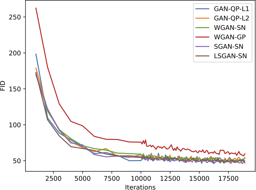
And the table below:
| GAN-QP-L1/L2 | WGAN-GP | WGAN-SN | SGAN-SN | LSGAN-SN | |
|---|---|---|---|---|---|
| Best FID | 45.0 / 44.7 | 55.5 | 47.8 | 44.5 | 45.8 |
| Speed | 1x / 1x | 1.5x | 1x | 1x | 1x |
256 and 512
At 128 resolution, the best performers were GAN-QP and SGAN-SN. However, at 256 \times 256 resolution, a gap appeared between them:
| GAN-QP | SGAN-SN | |
|---|---|---|
| Best FID | 22.7 | 27.9 |
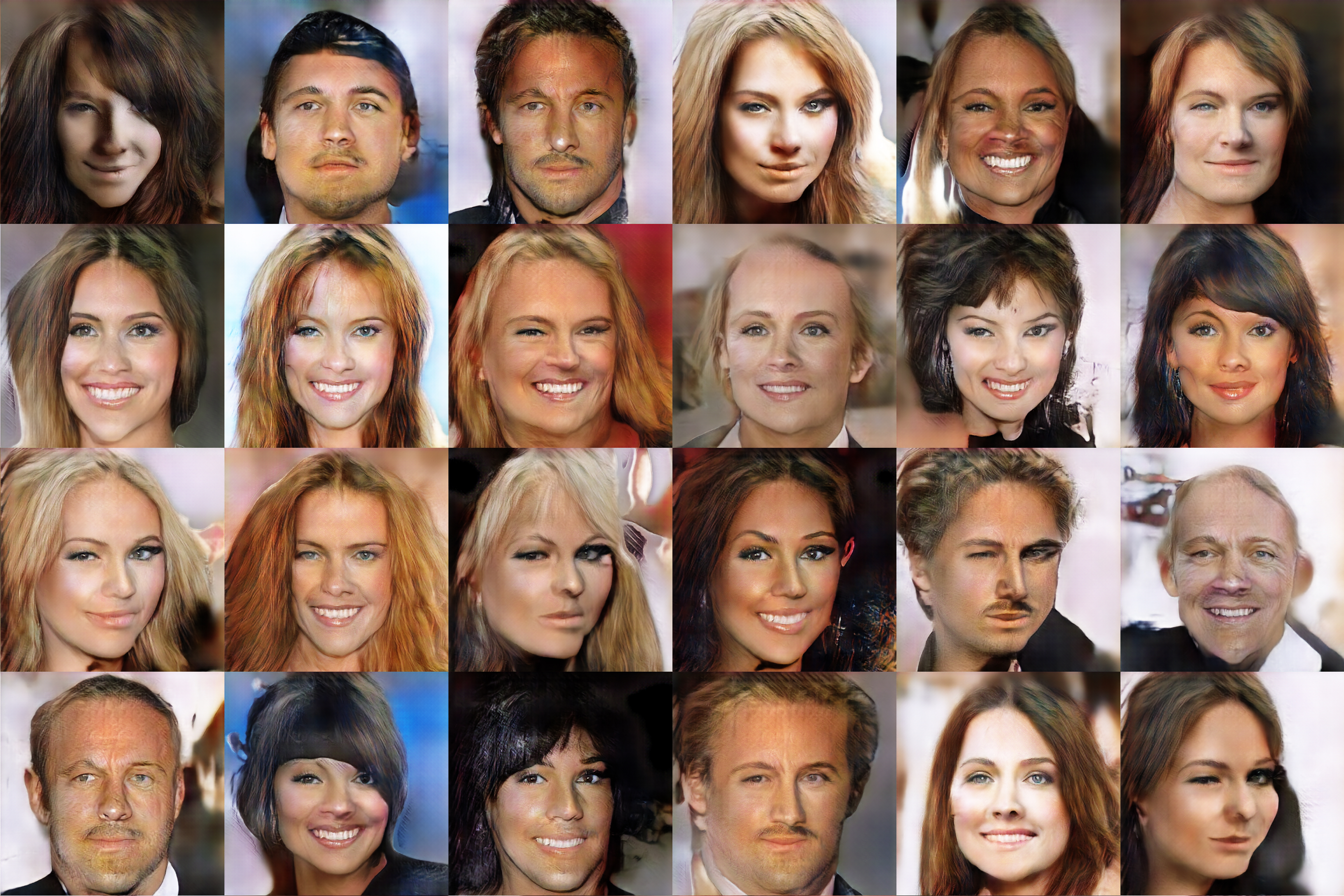
I pushed the GAN-QP experiments up to 512 \times 512 face generation, and the results were quite good, with a final FID of 26.44:
Summary
This article stems from my reflections on probability divergence, attempting to obtain a more direct scheme for understanding it, partly inspired by WGAN-div.
Fortunately, I was able to see this path through and obtained some new results, which I then submitted to arXiv for reference. I hope to receive guidance from experts and seniors. In fact, based on similar ideas, we can construct many similar divergences, such as replacing the square with 4th or 6th powers, though the theoretical analysis would become more difficult.
Due to limited computing power, and since I am not a dedicated GAN researcher, the experimental side might not be perfectly exhaustive. It is sufficient to demonstrate the conclusions. I hope everyone understands, and of course, I welcome your guidance.
When reposting, please include the original article address: https://kexue.fm/archives/6163