For Natural Language Processing (NLP), mutual information is a very important metric that measures the essential correlation between two entities. This blog has discussed mutual information multiple times, and I am quite interested in various articles that utilize it. A few days ago, I saw the recently proposed Deep INFOMAX model on Machine Heart (Ji Qi Zhi Xin). It uses the maximization of mutual information for unsupervised learning on images. Naturally, I was quite interested, and after studying it, I wrote this article.
The overall idea of this article originates from the original Deep INFOMAX paper, but I have not copied the original model exactly. Instead, I modified the model according to my own ideas (mainly the prior distribution part), and I will note these changes in the corresponding sections.
What Are We Doing?
Autoencoders
Feature extraction is a very important and fundamental task in unsupervised learning. A common form is training an encoder to encode the original dataset into a fixed-length vector. Naturally, our basic requirement for this encoder is: to retain (as much as possible) the important information of the original data.
How do we know if the encoding vector retains important information? A natural idea is that this encoding vector should also be able to reconstruct the original image. Therefore, we also train a decoder to attempt to reconstruct the original image, and the final loss is the Mean Squared Error (MSE) between the original image and the reconstructed image. This leads to the design of standard autoencoders. Later, we also hoped that the distribution of the encoding vectors would be as close to a Gaussian distribution as possible, which led to Variational Autoencoders (VAE).
Reflections on Reconstruction
However, it is worth considering whether the requirement of “reconstruction” is reasonable.
First, we can observe that the results of reconstructing the original image through low-dimensional encoding are usually very blurry. This can be explained by the fact that the MSE loss function is too harsh in requiring “pixel-by-pixel” reconstruction. Alternatively, it can be understood that for image reconstruction, we do not actually have a very suitable loss function to choose from. The most ideal method would be to use a Generative Adversarial Network (GAN) to train a discriminator, but this would further increase the difficulty of the task.
Secondly, an interesting fact is that most of us can distinguish between many real and counterfeit bills, but if we were asked to draw a hundred-yuan bill, I believe it would look almost nothing like the real thing. This indicates that for the task of identifying real and counterfeit bills, we can imagine having a pile of real and fake bills to learn from; we can extract very rich features from them, but these features are not sufficient to reconstruct the original image. They only allow us to distinguish the differences between these bills. In other words, for a dataset and a task, reasonable and sufficient features do not necessarily enable image reconstruction.
Maximizing Mutual Information
Mutual Information
The above discussion suggests that reconstruction is not a necessary condition for good features. The basic principle of a good feature should be “the ability to distinguish the sample from the entire dataset,” that is, extracting the (most) unique information of that sample. How do we measure whether the extracted information is unique to the sample? We use “mutual information” to measure it.
Let us first introduce some notation. Let X represent the set of original images, x \in X represent a specific original image, Z represent the set of encoding vectors, z \in Z represent a specific encoding vector, and p(z|x) represent the distribution of the encoding vector generated by x. We assume it is a Gaussian distribution, or simply understand it as the encoder we want to find. Then we can use mutual information to represent the correlation between X and Z: I(X,Z) = \iint p(z|x)\tilde{p}(x)\log \frac{p(z|x)}{p(z)}dxdz \label{eq:mi} Here, \tilde{p}(x) is the distribution of the original data, and p(z) is the distribution of the entire Z after p(z|x) is given, i.e., p(z) = \int p(z|x)\tilde{p}(x)dx A good feature encoder should maximize the mutual information, i.e., p(z|x) = \mathop{\text{argmax}}_{p(z|x)} I(X,Z) Larger mutual information means that (most of) \log \frac{p(z|x)}{p(z)} should be as large as possible. This means p(z|x) should be much larger than p(z); that is, for each x, the encoder can find a z that belongs exclusively to x, making the probability p(z|x) much larger than the random probability p(z). In this way, we have the ability to distinguish the original sample using only z.
Note: The name of [eq:mi] is mutual information, while the logarithmic term \log \frac{p(z|x)}{p(z)} is called “pointwise mutual information” (PMI), and sometimes simply referred to as mutual information. The difference between the two is: [eq:mi] calculates the overall relationship, such as answering the question “is there a relationship between the preceding and following words?”; \log \frac{p(z|x)}{p(z)} calculates a local relationship, such as answering the question “do the characters ’tan’ and ’te’ often appear together?”
Prior Distribution
As mentioned earlier, compared to autoencoders, Variational Autoencoders also hope that the latent variables follow a prior distribution of a standard normal distribution. This helps to make the encoding space more regular and even facilitates the decoupling of features for subsequent learning. Therefore, we also want to add this constraint here.
In the Deep INFOMAX paper, this constraint is added through adversarial training similar to the Adversarial Autoencoder (AAE) approach. However, it is well known that adversarial training is a minimax process that requires alternating training, which is not stable or concise enough. Here, I provide another more end-to-end approach: let q(z) be the standard normal distribution, and we minimize the KL divergence between p(z) and the prior distribution q(z): \label{eq:prior} KL(p(z)\Vert q(z))=\int p(z)\log \frac{p(z)}{q(z)}dz By combining [eq:mi] and [eq:prior] with weights, we get the total objective to be minimized: \begin{aligned} p(z|x) =& \min_{p(z|x)} \left\{- I(X,Z) + \lambda KL(p(z)\Vert q(z))\right\}\\ =&\min_{p(z|x)}\left\{-\iint p(z|x)\tilde{p}(x)\log \frac{p(z|x)}{p(z)}dxdz + \lambda\int p(z)\log \frac{p(z)}{q(z)}dz\right\} \end{aligned}\label{eq:total-loss-1} It looks very clear and beautiful, but we do not yet know the expression for p(z), so we cannot calculate it further. Thus, the matter is not yet finished.
Breaking It Down
Simplifying the Prior Term
Interestingly, by slightly transforming the loss in equation [eq:total-loss-1], we get: p(z|x) =\min_{p(z|x)}\left\{\iint p(z|x)\tilde{p}(x)\left[-(1+\lambda)\log \frac{p(z|x)}{p(z)} + \lambda \log \frac{p(z|x)}{q(z)}\right]dxdz\right\} Note that the above equation is exactly the weighted sum of mutual information and \mathbb{E}_{x\sim\tilde{p}(x)}[KL(p(z|x)\Vert q(z))]. Since the term KL(p(z|x)\Vert q(z)) can be calculated (it is exactly the KL divergence term in VAE), we have successfully solved half of the total loss, which can be written as: p(z|x) =\min_{p(z|x)}\left\{-\beta\cdot I(X,Z)+\gamma\cdot \mathbb{E}_{x\sim\tilde{p}(x)}[KL(p(z|x)\Vert q(z))]\right\}\label{eq:total-loss-2} Next, we focus on the mutual information term.
The Essence of Mutual Information
Now only the mutual information term remains. How can we maximize mutual information? Let’s slightly transform the definition of mutual information [eq:mi]: \begin{aligned} I(X,Z) =& \iint p(z|x)\tilde{p}(x)\log \frac{p(z|x)\tilde{p}(x)}{p(z)\tilde{p}(x)}dxdz\\ =& KL(p(z|x)\tilde{p}(x)\Vert p(z)\tilde{p}(x)) \end{aligned} This form reveals the essential meaning of mutual information: p(z|x)\tilde{p}(x) describes the joint distribution of the two variables x and z, while p(z)\tilde{p}(x) is the distribution when x and z are sampled independently (assuming they are uncorrelated). Mutual information is the KL divergence between these two distributions. Maximizing mutual information means increasing the distance between p(z|x)\tilde{p}(x) and p(z)\tilde{p}(x).
Note that KL divergence is theoretically unbounded. Maximizing an unbounded quantity is somewhat dangerous, as it could lead to infinite results. Therefore, for more effective optimization, we grasp the characteristic that “maximizing mutual information is increasing the distance between p(z|x)\tilde{p}(x) and p(z)\tilde{p}(x).” Instead of KL divergence, we use a bounded metric: Jensen-Shannon (JS) divergence (theoretically, Hellinger distance could also be used; please refer to “Introduction to f-GAN: The Production Workshop of GAN Models”). It is defined as: JS(P,Q) = \frac{1}{2}KL\left(P\left\Vert\frac{P+Q}{2}\right.\right)+\frac{1}{2}KL\left(Q\left\Vert\frac{P+Q}{2}\right.\right) JS divergence also measures the distance between two distributions, but it has an upper bound of \frac{1}{2}\log 2. When we maximize it, it achieves a similar effect to maximizing mutual information without worrying about the infinity problem. Thus, we replace equation [eq:total-loss-2] with the following objective: p(z|x) =\min_{p(z|x)}\left\{-\beta\cdot JS\big(p(z|x)\tilde{p}(x), p(z)\tilde{p}(x)\big)+\gamma\cdot \mathbb{E}_{x\sim\tilde{p}(x)}[KL(p(z|x)\Vert q(z))]\right\}\label{eq:total-loss-3} Of course, this does not change the essence or difficulty of the problem, as the JS divergence still hasn’t been calculated. Now we come to the final step of the breakthrough.
Conquering Mutual Information
In the article “Introduction to f-GAN: The Production Workshop of GAN Models”, we introduced the local variational inference for general f-divergence (equation (13) in that article): \mathcal{D}_f(P\Vert Q) = \max_{T}\Big(\mathbb{E}_{x\sim p(x)}[T(x)]-\mathbb{E}_{x\sim q(x)}[g(T(x))]\Big)\label{eq:f-div-e} For JS divergence, the result is: JS(P,Q) = \max_{T}\Big(\mathbb{E}_{x\sim p(x)}[\log \sigma(T(x))] + \mathbb{E}_{x\sim q(x)}[\log(1-\sigma(T(x))]\Big) Substituting p(z|x)\tilde{p}(x) and p(z)\tilde{p}(x) gives: \begin{aligned} &JS\big(p(z|x)\tilde{p}(x), p(z)\tilde{p}(x)\big)\\=& \max_{T}\Big(\mathbb{E}_{(x,z)\sim p(z|x)\tilde{p}(x)}[\log \sigma(T(x,z))] + \mathbb{E}_{(x,z)\sim p(z)\tilde{p}(x)}[\log(1-\sigma(T(x,z))]\Big) \end{aligned}\label{eq:f-div-e-js} You read that right; excluding the constant terms, it is completely equivalent to equation (5) in the Deep INFOMAX paper. I find it strange why the authors of the paper didn’t use this beautiful and intuitive form, but instead used a confusing one. In fact, the meaning of equation [eq:f-div-e-js] is very simple: it is “negative sampling estimation.” By introducing a discriminator network \sigma(T(x,z)), x and its corresponding z are treated as a positive sample pair, while x and a randomly sampled z are treated as a negative sample. Maximizing the likelihood function is equivalent to minimizing the cross-entropy.
In this way, through negative sampling, we provide a scheme for estimating JS divergence, and thus a scheme for estimating the JS version of mutual information, successfully conquering mutual information. Now, corresponding to equation [eq:total-loss-3], the specific loss is: \begin{aligned} &p(z|x),T(x,z) \\ =&\min_{p(z|x),T(x,z)}\Big\{-\beta\cdot\Big(\mathbb{E}_{(x,z)\sim p(z|x)\tilde{p}(x)}[\log \sigma(T(x,z))] + \mathbb{E}_{(x,z)\sim p(z)\tilde{p}(x)}[\log(1-\sigma(T(x,z))]\Big)\\ &\qquad\qquad\qquad+\gamma\cdot \mathbb{E}_{x\sim\tilde{p}(x)}[KL(p(z|x)\Vert q(z))]\Big\} \end{aligned}\label{eq:total-loss-4} Now, the theory is complete, and all that remains is to put it into practice.
From Global to Local
Shuffling Within the Batch
From an experimental perspective, how should equation [eq:total-loss-4] be operated? The KL divergence term for the prior distribution is not difficult; just follow the VAE approach. What about the mutual information term?
First, we randomly select an image x. Through the encoder, we obtain the mean and variance of z, and then reparameterize to get z_x. Such an (x, z_x) pair constitutes a positive sample. What about negative samples? To reduce the computational load, we directly shuffle the images within the batch and use the shuffled order as the basis for selecting negative samples. That is, if x was the 4th image in the original batch, and after shuffling, the 4th image is \hat{x}, then (x, z_x) is the positive sample and (\hat{x}, z_x) is the negative sample.
Local Mutual Information
The above approach actually considers the correlation between whole images. However, we know that image correlation is more reflected in local parts (which is why we use CNNs for images). In other words, image recognition, classification, etc., should be a process from local to global. Therefore, it is necessary to consider “local mutual information” as well.
The encoding process through a CNN is generally: \text{Original image } x \xrightarrow{\text{Multiple conv layers}} h \times w \times c \text{ features} \xrightarrow{\text{Conv and global pooling}} \text{Fixed-length vector } z We have already considered the correlation between x and z. What about the correlation between the intermediate layer features (feature map) and z? We denote the intermediate layer features as \{C_{ij}(x)|i=1,2,\dots,h; j=1,2,\dots,w\}, which we treat as a set of h \times w vectors. We also calculate the mutual information between these h \times w vectors and z_x, called “local mutual information.”
The estimation method is the same as the global one. Each C_{ij}(x) is concatenated with z_x to get [C_{ij}(x), z_x], which is equivalent to obtaining a larger feature map. Then, multiple 1 \times 1 convolutional layers are used on this feature map as the local mutual information estimation network T_{local}. The negative sample selection method also uses the shuffling scheme within the batch.
Now, the total loss including local mutual information is: \begin{aligned} &p(z|x),T_1(x,z),T_2(C_{ij}, z)=\min_{p(z|x),T_1,T_2}\Big\{\\ &\quad-\alpha\cdot\Big(\mathbb{E}_{(x,z)\sim p(z|x)\tilde{p}(x)}[\log \sigma(T_1(x,z))] + \mathbb{E}_{(x,z)\sim p(z)\tilde{p}(x)}[\log(1-\sigma(T_1(x,z))]\Big)\\ &\quad-\frac{\beta}{hw}\sum_{i,j}\Big(\mathbb{E}_{(x,z)\sim p(z|x)\tilde{p}(x)}[\log \sigma(T_2(C_{ij},z))] + \mathbb{E}_{(x,z)\sim p(z)\tilde{p}(x)}[\log(1-\sigma(T_2(C_{ij},z))]\Big)\\ &\quad+\gamma\cdot \mathbb{E}_{x\sim\tilde{p}(x)}[KL(p(z|x)\Vert q(z))]\Big\} \end{aligned}\label{eq:total-loss-5}
Other Information
In fact, there is much other information that can be considered.
For example, since we have considered the mutual information between C_{ij} and z, we can also consider the mutual information between C_{ij} themselves. That is, C_{ij} from the same image should be correlated, and their mutual information should be as large as possible (positive samples), while C_{ij} from different images should be uncorrelated, and their mutual information should be as small as possible. However, I have experimented with this, and the improvement was not particularly significant.
There is also multi-scale information. One can manually perform multi-scale data augmentation on the input images, or introduce multi-scale structures or Attention structures into the encoder. Such operations can be considered for inclusion in unsupervised learning to improve encoding quality.
Similarities to Word2Vec
In fact, readers familiar with the principles of the Word2Vec model in NLP will feel: Isn’t this just Word2Vec for images?
Indeed, in terms of principles and methods, Deep INFOMAX is largely the same as Word2Vec. In Word2Vec, negative samples are also randomly collected, and then a discriminator is used to distinguish between them. This process is usually called “Noise Contrastive Estimation” (NCE). As we mentioned before, the actual optimization objective of the NCE process (negative sampling) in Word2Vec is mutual information. (For details, please refer to “Talk on ’Noise Contrastive Estimation’: The Beauty of the Winding Path”).
In Word2Vec, a window size is fixed, and word co-occurrences are counted within the window (positive samples). What about Deep INFOMAX? Since there is only one image and no other “words,” it simply divides the image into small blocks and treats an image as a window, where each small block of the image is a word. Of course, to be more accurate, Deep INFOMAX is more like the Doc2Vec model, which is similar to Word2Vec.
From another perspective, it can also be understood this way: the introduction of local mutual information is equivalent to treating each small local part as a sample. This is equivalent to turning 1 sample into 1+hw samples, greatly increasing the sample size and thus improving the effect. At the same time, this ensures that every “corner” of the image is used. Because with low-dimensional compression encoding—for example, encoding 32 \times 32 \times 3 into 128 dimensions—it is very likely that an 8 \times 8 \times 3 > 128 area in the top-left corner could already uniquely identify the image. But this doesn’t represent the whole image, so we must find a way to use the entire image.
Open Source and Results
Reference Code
The implementation code for the above model is relatively simple (much easier than my reproduction of the Glow model!). It is not difficult regardless of the framework used. Below is a version implemented in Keras (Python 2.7 + Tensorflow 1.8 + Keras 2.2.4):
Behold, the Images
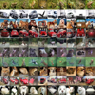
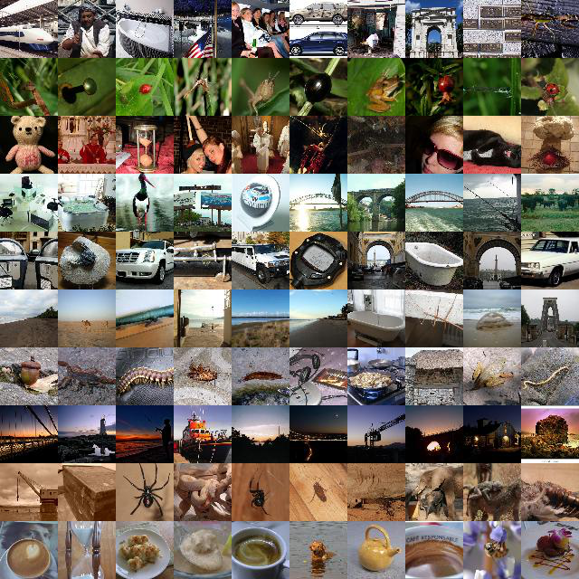
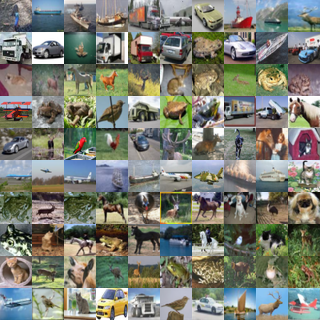
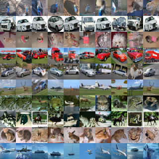
The quality of unsupervised algorithms is difficult to judge quantitatively. Generally, it is evaluated by looking at the performance on many downstream tasks. Just like when word vectors were very popular, how to quantitatively measure the quality of word vectors was a very headache-inducing problem. The Deep INFOMAX paper performed many related experiments, which I will not repeat here. Let’s just look at its K-Nearest Neighbors (KNN) effect (finding the k most similar images for a given image).
Overall, the results are satisfactory. I think after fine-tuning, it wouldn’t be a problem to use it for a simple image-based search. Many experimental results in the original paper were also good, further confirming the power of this idea.
CIFAR-10
In each row, the first image on the left is the original image, and the 9 images on the right are the nearest neighbors using cosine similarity. The results using Euclidean distance are similar.
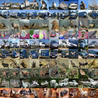
Tiny ImageNet
In each row, the first image on the left is the original image, and the 9 images on the right are the nearest neighbors using cosine similarity.
Global vs. Local
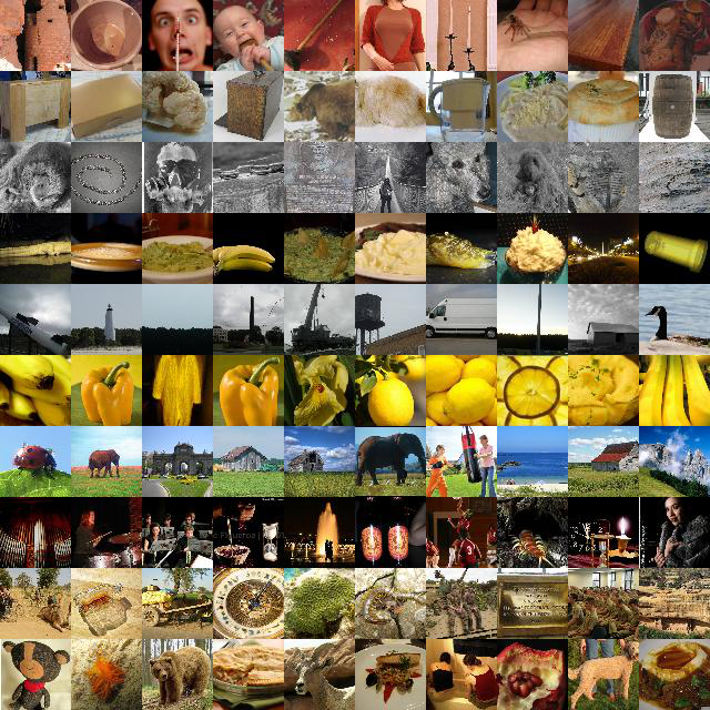
The introduction of local mutual information is very necessary. Below is a comparison of the KNN differences when using only global mutual information versus only local mutual information.
The Final Stop
As a success of unsupervised learning, the concept of mutual information, commonly found in NLP, has been generalized, theorized, and applied to images. Of course, it now seems that it can also be applied back to NLP or even other fields because it has been abstracted and has strong applicability.
I like the style of the entire Deep INFOMAX paper: from a generalized concept (maximizing mutual information) to an estimation framework and then to a practical model. The logic is clear and the demonstration is complete. It is the style of an ideal article in my mind (except for its use of adversarial networks for the prior distribution, which I believe is unnecessary). I look forward to seeing more articles of this type.
When reposting, please include the original address of this article: https://kexue.fm/archives/6024
For more detailed reposting matters, please refer to: “Scientific Space FAQ”