Lipschitz Constraints in Deep Learning: Generalization and Generative Models

Sensitivity to Perturbations

Let the input be x, the output be y, the model be f, and the model parameters be w, denoted as: y = f_w(x) Often, we hope to obtain a "robust" model. What does robust mean? Generally, it has two meanings. First is the stability with respect to parameter perturbations: for example, if the model changes to f_{w+\Delta w}(x), can it still achieve similar results? In dynamical systems, one also considers whether the model can eventually recover to f_w(x). Second is the stability with respect to input perturbations: for example, if the input changes from x to x+\Delta x, can f_w(x+\Delta x) provide a similar prediction? Readers may have heard that deep learning models are susceptible to "adversarial examples," where changing just one pixel in an image can lead to a completely different classification result. This is a case where the model is too sensitive to the input.

L-constraints

Thus, in most cases, we want the model to be insensitive to input perturbations, which usually improves the generalization performance of the model. That is, we want \| f_w(x_1) - f_w(x_2) \| to be as small as possible when \| x_1 - x_2 \| is very small. Of course, "as small as possible" is vague. Lipschitz proposed a more specific constraint: there exists a constant C (which depends only on the parameters and not on the input) such that the following inequality always holds: \| f_w(x_1) - f_w(x_2) \| \leq C(w) \cdot \| x_1 - x_2 \| \label{eq:l-cond} In other words, we want the entire model to be "controlled" by a linear function. This is the L-constraint.

In other words, we believe that a model satisfying the L-constraint is a good model. For a specific model, we want to estimate the expression of C(w) and hope that C(w) is as small as possible. A smaller C(w) means the model is less sensitive to input perturbations and has better generalization.

Neural Networks

Here we analyze specific neural networks to observe when they satisfy the L-constraint.

For simplicity, consider a single-layer fully connected network f(Wx+b), where f is the activation function and W, b are the parameter matrix and vector. Then [eq:l-cond] becomes: \| f(Wx_1+b) - f(Wx_2+b) \| \leq C(W,b) \cdot \| x_1 - x_2 \| If x_1 and x_2 are sufficiently close, we can approximate the left side with a first-order term: \left\| \frac{\partial f}{\partial y} W (x_1 - x_2) \right\| \leq C(W,b) \cdot \| x_1 - x_2 \| where y = Wx_2 + b. Obviously, for the left side not to exceed the right side, the absolute value of each element in the term \partial f / \partial y must not exceed a certain constant. This requires us to use activation functions with bounded derivatives. However, our commonly used activation functions, such as sigmoid, tanh, and ReLU, all satisfy this condition. Assuming the gradient of the activation function is already bounded (especially for ReLU, where the bound is 1), the \partial f / \partial y term only contributes a constant. We can temporarily ignore it and focus on \| W(x_1 - x_2) \|.

Multi-layer neural networks can be analyzed recursively, eventually reducing to the single-layer problem. Structures like CNNs and RNNs are essentially special cases of fully connected layers, so the same results apply. Therefore, for neural networks, the problem becomes: if \| W(x_1 - x_2) \| \leq C \| x_1 - x_2 \| \label{sec:l-cond-nn} holds constantly, what can the value of C be? Once we find the expression for C, we can aim to minimize it, thereby adding a regularization term C^2 to the parameters.

Definition

At this point, we have transformed the problem into a matrix norm problem (the matrix norm acts like the length of a vector). It is defined as: \| W \|_2 = \max_{x \neq 0} \frac{\| Wx \|}{\| x \|} \label{eq:m-norm} If W is a square matrix, this norm is also called the "spectral norm" or "spectral radius." In this article, even if it is not a square matrix, we will call it the "spectral norm." Note that \| Wx \| and \| x \| refer to vector norms, which are standard vector lengths. The matrix norm on the left is defined through the limit of the vector norms on the right, so this type of matrix norm is called a "matrix norm induced by vector norms."

Without getting bogged down in terminology, with the concept of vector norms, we have: \| W(x_1 - x_2) \| \leq \| W \|_2 \cdot \| x_1 - x_2 \| Essentially, we’ve just changed the notation; we still haven’t determined the value of \| W \|_2.

Frobenius Norm

The precise concept and calculation of the spectral norm \| W \|_2 involve significant linear algebra. Let’s first look at a simpler norm: the Frobenius norm, or F-norm.

Despite the intimidating name, its definition is simple: \| W \|_F = \sqrt{\sum_{i,j} w_{ij}^2} Simply put, it treats the matrix as a vector and calculates its Euclidean length.

Using the Cauchy-Schwarz inequality, we can easily prove: \| Wx \| \leq \| W \|_F \cdot \| x \| Clearly, \| W \|_F provides an upper bound for \| W \|_2. That is, while \| W \|_2 is the most accurate C in equation [sec:l-cond-nn] (the smallest C that satisfies it), if you don’t care about precision, you can simply use C = \| W \|_F to satisfy [sec:l-cond-nn], as \| W \|_F is easy to calculate.

L_2 Regularization

As mentioned, to make the neural network satisfy the L-constraint as much as possible, we want C = \| W \|_2 to be small. We can add C^2 as a regularization term to the loss function. Although we haven’t calculated the spectral norm \| W \|_2 yet, we have calculated a larger upper bound \| W \|_F. Let’s use that for now: loss = loss(y, f_w(x)) + \lambda \| W \|_F^2 \label{eq:l2-regular} where the first part is the original model loss. Looking at the expression for \| W \|_F, we see the added regularization term is: \lambda \left( \sum_{i,j} w_{ij}^2 \right) This is exactly L_2 regularization!

Finally, we have a reward for our efforts: we have revealed the connection between L_2 regularization (also known as weight decay) and L-constraints, showing that L_2 regularization helps the model satisfy L-constraints, thereby reducing sensitivity to input perturbations and enhancing generalization performance.

Principal Eigenvalue

Now we formally address the spectral norm \| W \|_2. This is a theoretical topic in linear algebra.

In fact, the spectral norm \| W \|_2 is equal to the square root of the largest eigenvalue (principal eigenvalue) of W^\top W. If W is a square matrix, then \| W \|_2 is equal to the absolute value of the largest eigenvalue of W.

Note: For readers interested in the theoretical proof, here is the general idea. According to definition [eq:m-norm]: \| W \|_2^2 = \max_{x \neq 0} \frac{x^\top W^\top W x}{x^\top x} = \max_{\| x \|=1} x^\top W^\top W x Assume W^\top W is diagonalized as \text{diag}(\lambda_1, \dots, \lambda_n), i.e., W^\top W = U^\top \text{diag}(\lambda_1, \dots, \lambda_n) U, where \lambda_i are its eigenvalues (all non-negative) and U is an orthogonal matrix. Since the product of an orthogonal matrix and a unit vector is still a unit vector: \begin{aligned} \| W \|_2^2 &= \max_{\| x \|=1} x^\top \text{diag}(\lambda_1, \dots, \lambda_n) x \\ &= \max_{\| x \|=1} (\lambda_1 x_1^2 + \dots + \lambda_n x_n^2) \\ &\leq \max\{\lambda_1, \dots, \lambda_n\} (x_1^2 + \dots + x_n^2) \quad (\text{since } \| x \|=1) \\ &= \max\{\lambda_1, \dots, \lambda_n\} \end{aligned} Thus, \| W \|_2^2 equals the largest eigenvalue of W^\top W.

Power Iteration

Some readers might be getting impatient: "Who cares if it’s an eigenvalue? I just want to know how to calculate this norm!"

Actually, the previous content is the foundation for calculating \| W \|_2. Since \| W \|_2^2 is the largest eigenvalue of W^\top W, the problem becomes finding that eigenvalue, which can be solved using the "Power Iteration" method.

Power iteration uses the following iterative format: u \leftarrow \frac{(W^\top W)u}{\| (W^\top W)u \|} After several iterations, the norm is approximated by: \| W \|_2^2 \approx u^\top W^\top W u This can be equivalently rewritten as: v \leftarrow \frac{W^\top u}{\| W^\top u \|}, \quad u \leftarrow \frac{Wv}{\| Wv \|}, \quad \| W \|_2 \approx u^\top Wv \label{eq:m-norm-iter} After initializing u, v (e.g., with all-ones vectors), you can iterate a few times to get u, v, and then calculate the approximate \| W \|_2 using u^\top Wv.

Note: For interested readers, here is a simple proof of why this iteration works.

Let A = W^\top W, initialized with u^{(0)}. Assume A is diagonalizable and its largest eigenvalue \lambda_1 is strictly greater than the others. The eigenvectors \eta_1, \dots, \eta_n form a complete basis, so we can write: u^{(0)} = c_1 \eta_1 + \dots + c_n \eta_n The iteration is Au / \| Au \|. Ignoring the normalization for a moment and looking at the repeated application of A: A^r u^{(0)} = c_1 A^r \eta_1 + \dots + c_n A^r \eta_n Since A\eta = \lambda \eta: A^r u^{(0)} = c_1 \lambda_1^r \eta_1 + \dots + c_n \lambda_n^r \eta_n Assuming \lambda_1 is the largest eigenvalue: \frac{A^r u^{(0)}}{\lambda_1^r} = c_1 \eta_1 + c_2 \left(\frac{\lambda_2}{\lambda_1}\right)^r \eta_2 + \dots + c_n \left(\frac{\lambda_n}{\lambda_1}\right)^r \eta_n Since \lambda_i / \lambda_1 < 1 for i > 1, as r \to \infty, these terms tend to zero. Thus: \frac{A^r u^{(0)}}{\lambda_1^r} \approx c_1 \eta_1 This shows that for large r, A^r u^{(0)} points in the direction of the principal eigenvector. The normalization at each step prevents overflow. Thus u = A^r u^{(0)} / \| A^r u^{(0)} \| is the unit principal eigenvector, i.e., Au = \lambda_1 u. Therefore: u^\top A u = \lambda_1 u^\top u = \lambda_1 This yields the square of the spectral norm.

Spectral Regularization

We have shown the relationship between the Frobenius norm and L_2 regularization, and noted that the Frobenius norm is a coarser condition. The more accurate norm is the spectral norm. Although it is harder to calculate, it can be approximated using a few steps of equation [eq:m-norm-iter].

Thus, we can propose the concept of "Spectral Norm Regularization", using the square of the spectral norm as an additional regularization term instead of simple L_2 regularization. Equation [eq:l2-regular] becomes: loss = loss(y, f_w(x)) + \lambda \| W \|_2^2

The paper "Spectral Norm Regularization for Improving the Generalizability of Deep Learning" conducted several experiments showing that spectral regularization improves model performance across various tasks.

In Keras, the spectral norm can be calculated with the following code:

def spectral_norm(w, r=5):
    w_shape = K.int_shape(w)
    in_dim = np.prod(w_shape[:-1]).astype(int)
    out_dim = w_shape[-1]
    w = K.reshape(w, (in_dim, out_dim))
    u = K.ones((1, in_dim))
    for i in range(r):
        v = K.l2_normalize(K.dot(u, w))
        u = K.l2_normalize(K.dot(v, K.transpose(w)))
    return K.sum(K.dot(K.dot(u, w), K.transpose(v)))

WGAN

If L-constraints are just "the icing on the cake" for supervised learning, they are a critical step for the WGAN discriminator. The optimization objective of the WGAN discriminator is: W(P_r, P_g) = \sup_{|f|_L = 1} \mathbb{E}_{x \sim P_r}[f(x)] - \mathbb{E}_{x \sim P_g}[f(x)] where P_r, P_g are the real and generated distributions, and |f|_L = 1 denotes the Lipschitz constraint |f(x_1) - f(x_2)| \leq \| x_1 - x_2 \| (where C=1). The objective is to find the function f that satisfies this constraint and maximizes the difference in expectations. In loss form: \min_{|f|_L = 1} \mathbb{E}_{x \sim P_g}[f(x)] - \mathbb{E}_{x \sim P_r}[f(x)]

Gradient Penalty

One effective solution currently is gradient penalty, where \| f'(x) \| = 1 is a sufficient condition for |f|_L = 1. This is added to the discriminator loss as a penalty: \min_{f} \mathbb{E}_{x \sim P_g}[f(x)] - \mathbb{E}_{x \sim P_r}[f(x)] + \lambda (\| f'(x_{inter}) \| - 1)^2 In fact, I think adding a relu(x) = \max(x, 0) might be better: \min_{f} \mathbb{E}_{x \sim P_g}[f(x)] - \mathbb{E}_{x \sim P_r}[f(x)] + \lambda \max(\| f'(x_{inter}) \| - 1, 0)^2 where x_{inter} is obtained via random interpolation: \begin{aligned} &x_{inter} = \varepsilon x_{real} + (1 - \varepsilon) x_{fake} \\ &\varepsilon \sim U[0,1], \quad x_{real} \sim P_r, \quad x_{fake} \sim P_g \end{aligned} Gradient penalty doesn’t guarantee \| f'(x) \| = 1, but intuitively it fluctuates around 1, so |f|_L theoretically fluctuates around 1, approximating the L-constraint.

This scheme works well in many cases, but performs poorly when the number of real sample classes is large (especially in conditional generation). The problem lies in random interpolation: in principle, the L-constraint must be satisfied throughout the entire space, but gradient penalty via linear interpolation only ensures it in a small region. If this region happens to be the space between real and generated samples, it’s barely enough. However, with many classes, interpolating between different classes often lands in unknown regions, failing to satisfy the L-condition where needed, causing the discriminator to fail.

Thought: Can gradient penalty be used directly as a regularization term for supervised models? Interested readers can try it out.

Spectral Normalization

The problem with gradient penalty is that it is just a penalty and only works locally. A truly ingenious solution is the construction method: build a special f such that it satisfies the L-constraint regardless of its parameters.

When WGAN was first proposed, it used weight clipping—clipping the absolute values of all parameters to a constant. This ensures the Frobenius norm doesn’t exceed a constant, so |f|_L doesn’t exceed a constant. While it doesn’t strictly implement |f|_L = 1, it only scales the loss by a constant, which doesn’t affect optimization. Weight clipping is a construction method, but it is not very friendly to optimization.

There is much room for improvement. For example, one could clip the Frobenius norm of all parameters. This provides more flexibility than direct weight clipping. If clipping is too crude, parameter penalty is an alternative—applying a large penalty to parameters whose Frobenius norm exceeds a threshold. I’ve tested this; it works but converges slowly.

However, these are all approximations. Now that we have the spectral norm, we can use the most precise solution: replace all parameters w in f with w / \| w \|_2. This is Spectral Normalization, proposed and experimented with in "Spectral Normalization for Generative Adversarial Networks". If the absolute values of the derivatives of the activation functions used in f do not exceed 1, then we have |f|_L \leq 1, achieving the required L-constraint precisely.

Note: The condition "absolute values of derivatives of activation functions do not exceed 1" is usually met. However, if the discriminator uses a residual structure, the activation is effectively x + relu(Wx+b), where the derivative might exceed 1. Regardless, it will not exceed a constant, so it doesn’t affect optimization.

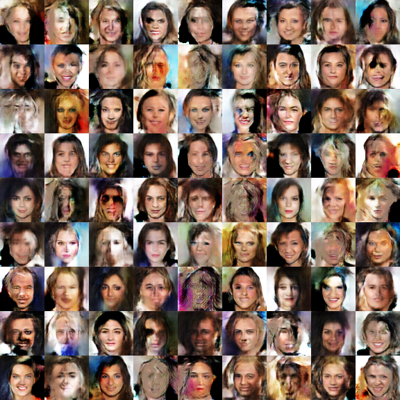
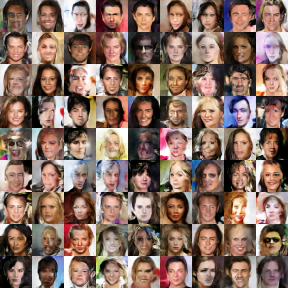
I have tried using spectral normalization in WGAN (without gradient penalty; see the reference code below) and found that the final convergence speed (epochs needed for the same effect) is faster than WGAN-GP, and the results are slightly better. Furthermore, there is another reason for the speed: the execution time per epoch is shorter than with gradient penalty. With gradient penalty, the second-order gradient must be calculated during descent, requiring the entire forward pass to be executed twice, which is slower.

Keras Implementation

Implementing spectral normalization in Keras can be described as both simple and not simple.

It is simple because you only need to pass the kernel_constraint parameter to every convolutional and fully connected layer in the discriminator, and the gamma_constraint to BN layers. The constraint is written as:

def spectral_normalization(w):
    return w / spectral_norm(w)

Reference code: https://github.com/bojone/gan/blob/master/keras/wgan_sn_celeba.py

It is "not simple" because in current Keras (version 2.2.4), kernel_constraint does not actually change the kernel during the forward pass; it only adjusts the kernel values after gradient descent. This differs from the spectral normalization method in the paper. If used this way, you will find that gradients become inaccurate in later stages, and generation quality suffers. To truly modify the kernel, one must either redefine all layers (Conv, Dense, BN, etc.) or modify the source code. Modifying the source code is the simplest solution. Modify the add_weight method of the Layer object in keras/engine/base_layer.py (starting around line 222):

    def add_weight(self,
                   name,
                   shape,
                   dtype=None,
                   initializer=None,
                   regularizer=None,
                   trainable=True,
                   constraint=None):
        # ... (docstring omitted)
        initializer = initializers.get(initializer)
        if dtype is None:
            dtype = K.floatx()
        weight = K.variable(initializer(shape),
                            dtype=dtype,
                            name=name,
                            constraint=constraint)
        # ...

Change it to:

    def add_weight(self,
                   name,
                   shape,
                   dtype=None,
                   initializer=None,
                   regularizer=None,
                   trainable=True,
                   constraint=None):
        # ... (docstring omitted)
        initializer = initializers.get(initializer)
        if dtype is None:
            dtype = K.floatx()
        weight = K.variable(initializer(shape),
                            dtype=dtype,
                            name=name,
                            constraint=None)
        if regularizer is not None:
            with K.name_scope('weight_regularizer'):
                self.add_loss(regularizer(weight))
        if trainable:
            self._trainable_weights.append(weight)
        else:
            self._non_trainable_weights.append(weight)
        if constraint is not None:
            return constraint(weight)
        return weight

Essentially, change the constraint in K.variable to None and execute the constraint at the very end. Note: Don’t immediately complain that Keras is too rigid or inflexible because you have to modify the source code. If you were using other frameworks, the modifications would likely be many times more complex (relative to the amount of change for a GAN without spectral normalization).

(Update: A new implementation method that does not require modifying the source code can be found here.)