This article is the English version of the paper we recently posted on arXiv. In this paper, we present an approach to combine flow models (such as the previously introduced Glow) with Variational Autoencoders (VAEs), which we call f-VAEs. Theoretically, it can be proven that f-VAEs constitute a more general framework encompassing both flow models and VAEs. Experiments show that compared to the original Glow model, f-VAEs converge faster and can achieve the same generation quality with a smaller network scale.
Original paper: "f-VAEs: Improve VAEs with Conditional Flows"
Recently, generative models have received widespread attention. Among them, Variational Autoencoders (VAEs) and flow models are two types of generative models distinct from Generative Adversarial Networks (GANs), and they have also been extensively studied. However, each has its own advantages and disadvantages. This article attempts to combine them.
Basics
Let the evidence distribution of a given dataset be \tilde{p}(x). The basic idea of generative models is to fit the dataset distribution using the following distribution form: q(x)=\int q(z)q(x|z) dz where q(z) is generally a standard Gaussian distribution, and q(x|z) is typically a Gaussian distribution (in VAEs) or a Dirac distribution (in GANs and flow models). Ideally, the optimization method is to maximize the likelihood function \mathbb{E}[\log q(x)], or equivalently, minimize KL(\tilde{p}(x)\Vert q(x)).
Since the integral may be difficult to calculate explicitly, special solving techniques are required, leading to different generative models. Among them, VAE introduces a posterior distribution p(z|x) and changes the optimization target to a more easily calculated upper bound KL(\tilde{p}(x)p(z|x)\Vert q(z)q(x|z)). As is well known, VAE has advantages such as fast convergence and stable training, but in general, the generated images suffer from issues like blurriness, the reasons for which we will discuss later.
In flow models, q(x|z)=\delta(x - G(z)), and G(z) is carefully designed (through a composition of flows) to calculate this integral directly. The main component of a flow model is the "coupling layer": first, x is partitioned into two parts x_1, x_2, and then the following operations are performed: \begin{aligned} y_1 &= x_1\\ y_2 &= s(x_1)\otimes x_2 + t(x_1) \end{aligned} \label{eq:coupling} This transformation is reversible, and the inverse transformation is: \begin{aligned} x_1 &= y_1\\ x_2 &= (y_2 - t(y_1)) / s(x_1) \end{aligned} Its Jacobian determinant is \prod_i s_i(x_i). This transformation is usually called "affine coupling" (if s(x_1)\equiv 1, it is usually called "additive coupling"), denoted by f. By combining many coupling layers, we can obtain complex non-linear transformations, i.e., G = f_1 \circ f_2 \circ \dots \circ f_n. This is what is known as an (unconditional) flow.
Because the integral is calculated directly, flow models can directly perform maximum likelihood optimization. The recently released Glow model has shown powerful generation effects, attracting much discussion and attention. However, flow models are usually quite massive and take a long time to train (for example, the 256\times 256 image generation model was trained for a week on 40 GPUs), which is clearly not friendly enough.
Analysis
There are many explanations for the blurriness of images generated by VAEs. Some believe it is a problem with the MSE error, while others believe it is an inherent property of the KL divergence. However, it is worth noting that even if the KL divergence term for the latent variable is removed, turning it into a standard autoencoder, the reconstructed images are usually still blurry. This suggests that image blurriness in VAEs may be an inherent problem of low-dimensional reconstruction of the original image.
What if the latent variable dimension is set to be the same as the input dimension? That still seems insufficient because standard VAEs assume the posterior distribution is Gaussian. This limits the model’s expressive power because the Gaussian distribution family is only a tiny part of all possible posterior distributions. If the nature of the posterior distribution is far from Gaussian, the fitting effect will be poor.
What is the problem with flow models like Glow? Flow models transform the input distribution into a Gaussian distribution by designing a reversible (strongly non-linear) transformation. In this process, not only must the reversibility of the transformation be guaranteed, but its Jacobian determinant must also be easy to calculate. This leads to the design of "additive coupling layers" or "affine coupling layers." However, these coupling layers only provide very weak non-linear capabilities, so a sufficient number of coupling layers are needed to accumulate into a strong non-linear transformation. Consequently, Glow models are usually large and require long training times.
f-VAEs
Our approach is to introduce flow models into VAEs, using flow models to fit a more general posterior distribution p(z|x) instead of simply setting it as a Gaussian distribution. We call this f-VAEs (Flow-based Variational Autoencoders). Compared to standard VAEs, f-VAEs break through the limitation of the posterior distribution being Gaussian, ultimately allowing VAEs to generate sharp images. Compared to original flow models (like Glow), the encoder in f-VAEs brings stronger non-linear capabilities to the model, thereby reducing the reliance on coupling layers and achieving the same generation effect with a smaller model scale.
Derivation Process
We start from the original objective of VAEs. The VAE loss can be written as: \begin{aligned} &KL(\tilde{p}(x)p(z|x)\Vert q(z)q(x|z))\\ =&\iint \tilde{p}(x)p(z|x)\log \frac{\tilde{p}(x)p(z|x)}{q(x|z)q(z)} dzdx \end{aligned} \label{eq:vae-loss} where p(z|x) and q(x|z) are both distributions with parameters. Unlike standard VAEs, p(z|x) is no longer assumed to be Gaussian but is constructed through a flow model: p(z|x) = \int \delta(z - F_x(u))q(u)du \label{eq:cond-flow} Here q(u) is a standard Gaussian distribution, and F_x(u) is a binary function of x and u, but it is reversible with respect to u. It can be understood as a flow model for u, but its parameters may depend on x. We call this a "conditional flow." Substituting into [eq:vae-loss] yields: \iint \tilde{p}(x)q(u)\log \frac{\tilde{p}(x) q(u)}{q(x| F_x(u))q(F_x(u))\left|\det \left[\frac{\partial F_x (u)}{\partial u}\right]\right|} dudx \label{eq:f-vae-loss} This is the loss for a general f-VAE.
Derivation: Combining [eq:vae-loss] and [eq:cond-flow], we have: \begin{aligned} &\iiint \tilde{p}(x)\delta(z - F_x(u))q(u)\log \frac{\tilde{p}(x)\int\delta(z - F_x(u'))q(u')du'}{q(x|z)q(z)} dzdudx\\ =&\iint \tilde{p}(x)q(u)\log \frac{\tilde{p}(x)\int\delta(F_x(u) - F_x(u'))q(u')du'}{q(x| F_x(u))q(F_x(u))} dudx \end{aligned} \label{eq:vae-loss-cond-flow} Let v = F_x(u'), so u'=H_x(v). For the Jacobian determinant, we have the relationship: \det \left[\frac{\partial u'}{\partial v}\right]=1\Big/\det \left[\frac{\partial v}{\partial u'}\right]=1\Big/\det \left[\frac{\partial F_x (u')}{\partial u'}\right] Thus [eq:vae-loss-cond-flow] becomes: \begin{aligned} &\iint \tilde{p}(x)q(u)\log \frac{\tilde{p}(x)\int\delta(F_x(u) - v)q(H_x(v))\left|\det \left[\frac{\partial u'}{\partial v}\right]\right|dv}{q(x| F_x(u))q(F_x(u))} dudx\\ =&\iint \tilde{p}(x)q(u)\log \frac{\tilde{p}(x) q(H_x(F_x(u)))\Big/\left|\det \left[\frac{\partial F_x (u')}{\partial u'}\right]\right|_{v=F_x(u)}}{q(x| F_x(u))q(F_x(u))} dudx\\ =&\iint \tilde{p}(x)q(u)\log \frac{\tilde{p}(x) q(u)}{q(x| F_x(u))q(F_x(u))\left|\det \left[\frac{\partial F_x (u)}{\partial u}\right]\right|} dudx \end{aligned}
Two Special Cases
Equation [eq:f-vae-loss] describes a generalized framework, and different F_x(u) correspond to different generative models. If we set: F_x(u)=\sigma(x)\otimes u + \mu(x) Then we have: -\int q(u)\log \left|\det \left[\frac{\partial F_x (u)}{\partial u}\right]\right| du=-\sum_i\log \sigma_i(x) and \int q(u)\log \frac{q(u)}{q(F_x(u))}du=\frac{1}{2}\sum_{i=1}^d(\mu_i^2(x)+\sigma_i^2(x)-1) Combining these two terms yields exactly the KL divergence between the posterior and prior distributions; substituting into [eq:f-vae-loss] gives the standard VAE loss. Surprisingly, this result automatically includes the reparameterization process.
Another simple example is: F_x(u)=F(\sigma u + x),\quad q(x|z)=\mathcal{N}(x;F^{-1}(z),\sigma^2) where \sigma is a small constant and F is any flow model with parameters independent of x (unconditional flow). In this case: -\log q(x|F_x(u)) = \frac{d}{2}\log 2\pi \sigma^2 + \frac{1}{2}\Vert u\Vert^2 The part of the loss containing trainable parameters becomes: -\iint \tilde{p}(x)q(u)\log q(F(\sigma u + x))\left|\det \left[\frac{\partial F(\sigma u + x)}{\partial u}\right]\right| dudx This is equivalent to a standard flow model where the input is augmented with Gaussian noise of variance \sigma^2. Interestingly, the standard Glow model does indeed add a certain amount of noise to the input images during training.
Our Model
The two special cases above show that [eq:f-vae-loss] in principle encompasses both VAEs and flow models. F_x(u) describes different ways of mixing u and x. We can choose any complex F_x(u) to improve the expressive power of the posterior distribution.
For image generation, considering that low-dimensional reconstruction leads to blurriness, we choose the dimension of z to be the same as x. We combine the previous ideas and select: F_x(u)=F(\sigma_1 u + E(x)),\quad q(x|z)=\mathcal{N}(x;G(F^{-1}(z)),\sigma_2^2) where \sigma_1, \sigma_2 are trainable parameters, E(\cdot) and G(\cdot) are the encoder and decoder, and F(\cdot) is an unconditional flow. The equivalent loss is: \begin{aligned} \iint \tilde{p}(x)q(u)\bigg[ & \frac{1}{2\sigma_2^2}\Vert G(\sigma_1 u + E(x))-x\Vert^2 + \frac{1}{2}F^2(\sigma_1 u + E(x)) \\ & \quad -\log \left|\det \left[\frac{\partial F(\sigma_1 u + E(x))}{\partial u}\right]\right|\bigg] dudx \end{aligned} The generation process is: u \sim q(u), z = F^{-1}(u), x = G(z).
Experiments
We conducted experiments on CelebA HQ at 64\times 64 and 128\times 128 resolutions.
Experimental Setup
The encoder E(\cdot) consists of convolutional layers and Squeeze operators. Each block uses residual steps x + CNN(x). The decoder G(\cdot) is the inverse structure of E(\cdot). The unconditional flow F(\cdot) follows the Glow architecture but with fewer layers and filters.
Source code: https://github.com/bojone/flow/blob/master/f-VAEs.py
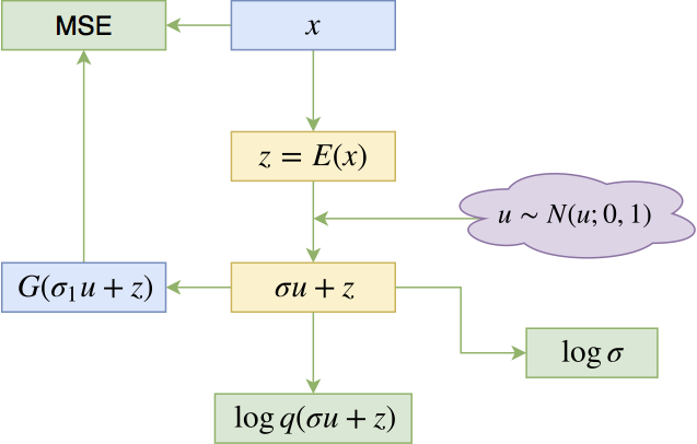
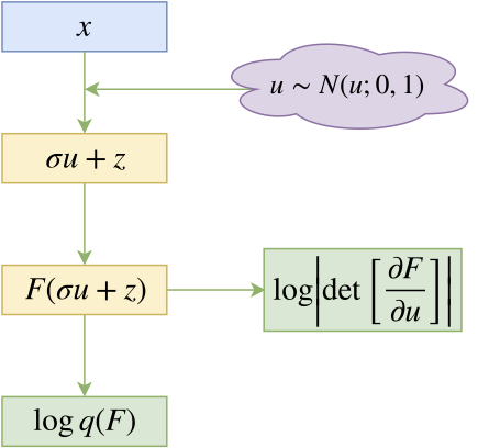
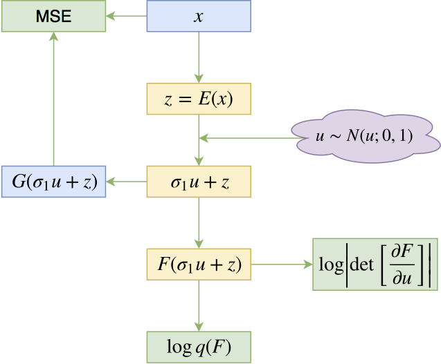
Experimental Results
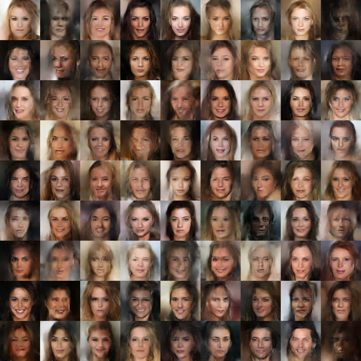
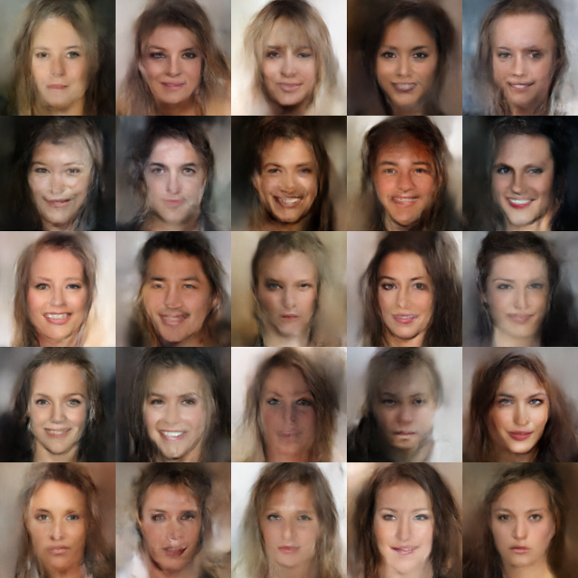
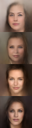
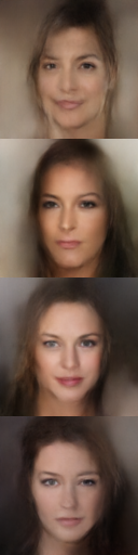
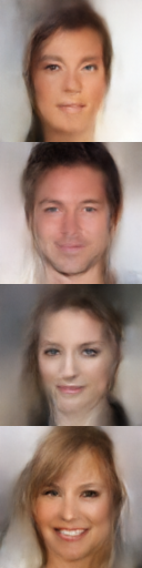
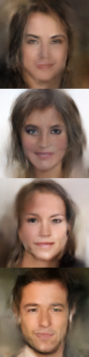
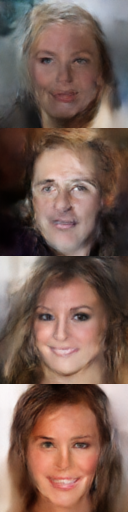
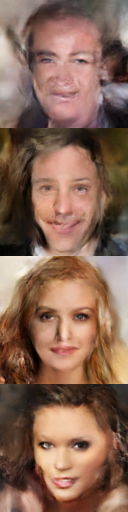
f-VAEs largely solve the blurriness problem of VAEs. Compared to Glow of the same scale, f-VAEs perform better within the same number of epochs. Training a 64\times 64 model takes about 7–8 hours on a GTX 1060.
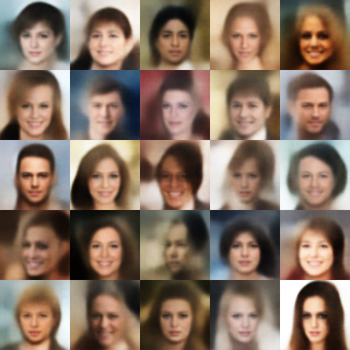
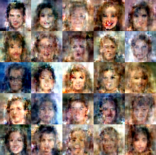
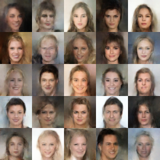
Random Sampling Results (128\times 128)
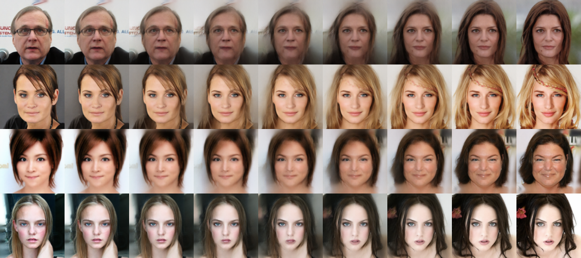
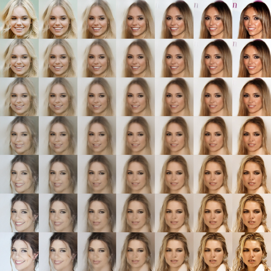
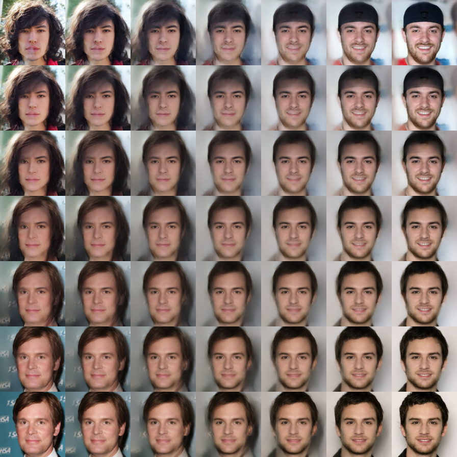
Latent Variable Linear Interpolation
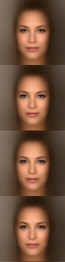
Effect of Annealing Parameter T
Conclusion
Our work addresses two issues with Glow: reducing computation and enabling dimensionality reduction. f-VAEs act as a "mini Glow" that achieves good results without requiring the full complexity of Glow’s flow layers. We also theoretically unified VAEs and flows into a single framework. Future work includes designing better encoders/decoders to improve detail and reduce the "oil painting" effect.
Original Address: https://kexue.fm/archives/5977