Variational Autoencoders (IV): A One-Step Clustering Scheme

General Framework

Recall the loss function of a VAE (if you need a refresher, please refer to “Variational Autoencoders (II): From a Bayesian Perspective”): KL\Big(p(x,z)\Big\Vert q(x,z)\Big) = \iint p(z|x)\tilde{p}(x)\ln \frac{p(z|x)\tilde{p}(x)}{q(x|z)q(z)} dzdx \tag{1} Typically, we assume that q(z) is a standard normal distribution, and p(z|x), q(x|z) are conditional normal distributions. Substituting these into the equation yields the standard VAE loss.

However, there is no rule stating that latent variables must be continuous. Here, we define the latent variables as (z, y), where z is a continuous variable representing the encoding vector, and y is a discrete variable representing the category. Replacing z in (1) with (z, y), we get: KL\Big(p(x,z,y)\Big\Vert q(x,z,y)\Big) = \sum_y \iint p(z,y|x)\tilde{p}(x)\ln \frac{p(z,y|x)\tilde{p}(x)}{q(x|z,y)q(z,y)} dzdx \tag{2} This is the loss function for a VAE used for clustering.

Step-by-step Assumptions

Is that it? Well, yes. If we only consider the generalized framework, equation (2) is indeed the conclusion.

However, in practice, (2) can be implemented in many different ways. Here we introduce a relatively simple one. First, we must clarify that in (2), we only know \tilde{p}(x) (the empirical distribution given by a batch of data); the others are not explicitly defined. To solve (2), we need to set some forms. One selection scheme is: p(z,y|x)=p(y|z)p(z|x),\quad q(x|z,y)=q(x|z),\quad q(z,y)=q(z|y)q(y) \tag{3} Substituting these into (2) gives: KL\Big(p(x,z,y)\Big\Vert q(x,z,y)\Big) = \sum_y \iint p(y|z)p(z|x)\tilde{p}(x)\ln \frac{p(y|z)p(z|x)\tilde{p}(x)}{q(x|z)q(z|y)q(y)} dzdx \tag{4} Equation (4) is actually quite intuitive. It describes the encoding and generation processes:

1. Sample x from the original data, obtain the encoded feature z through p(z|x), and then classify the encoded feature through the classifier p(y|z) to obtain the category.

2. Select a category y from the distribution q(y), then select a random latent variable z from the distribution q(z|y), and finally decode it into the original sample through the generator q(x|z).

Specific Model

Equation (4) is already quite specific. We only need to follow the usual VAE practices: p(z|x) is generally assumed to be a normal distribution with mean \mu(x) and variance \sigma^2(x); q(x|z) is generally assumed to be a normal distribution with mean G(z) and constant variance (equivalent to using MSE as the loss); q(z|y) can be assumed to be a normal distribution with mean \mu_y and variance 1. As for the remaining q(y) and p(y|z), q(y) can be assumed to be a uniform distribution (it is a constant), which implies a hope that each class is roughly balanced, while p(y|z) is a classifier for the latent variables, which can be fitted using any softmax network.

Finally, we can visually rewrite (4) as: \mathbb{E}_{x\sim\tilde{p}(x)}\Big[-\log q(x|z) + \sum_y p(y|z) \log \frac{p(z|x)}{q(z|y)} + KL\big(p(y|z)\big\Vert q(y)\big)\Big],\quad z\sim p(z|x) \tag{5} Where z\sim p(z|x) is the reparameterization trick, and the three loss terms in the brackets each have their own meaning:

1. -\log q(x|z) hopes that the reconstruction error is as small as possible, meaning z should retain complete information.

2. \sum_y p(y|z) \log \frac{p(z|x)}{q(z|y)} hopes that z can align as much as possible with the “exclusive” normal distribution of a certain category; this step performs the clustering.

3. KL\big(p(y|z)\big\Vert q(y)\big) hopes that the distribution of each class is as balanced as possible, preventing two classes from overlapping almost entirely (collapsing into one class). Of course, sometimes this prior requirement might not be necessary, and this term can be removed.

Code Implementation

The code is located at: https://github.com/bojone/vae/blob/master/vae_keras_cluster.py

The comments should be quite clear, and there are few changes compared to a standard VAE. The part that might be slightly difficult is how to implement \sum_y p(y|z) \log \frac{p(z|x)}{q(z|y)}. First, we substitute: \begin{aligned} p(z|x)&=\frac{1}{\prod\limits_{i=1}^d\sqrt{2\pi\sigma_i^2(x)}}\exp\left\{-\frac{1}{2}\left\Vert\frac{z - \mu(x)}{\sigma(x)}\right\Vert^2\right\}\\ q(z|y)&=\frac{1}{(2\pi)^{d/2}}\exp\left\{-\frac{1}{2}\left\Vert z - \mu_y\right\Vert^2\right\} \end{aligned} \tag{6} to get: \log \frac{p(z|x)}{q(z|y)}=-\frac{1}{2}\sum_{i=1}^d \log \sigma_i^2(x)-\frac{1}{2}\left\Vert\frac{z - \mu(x)}{\sigma(x)}\right\Vert^2 + \frac{1}{2}\left\Vert z - \mu_y\right\Vert^2 \tag{7} Note that the second term is actually redundant because the reparameterization trick tells us z = \varepsilon\otimes \sigma(x) + \mu(x),\,\varepsilon\sim \mathcal{N}(0,1), so the second term is actually just -\Vert \varepsilon\Vert^2/2, which is independent of the parameters. Therefore: \log \frac{p(z|x)}{q(z|y)}\sim -\frac{1}{2}\sum_{i=1}^d \log \sigma_i^2(x) + \frac{1}{2}\left\Vert z - \mu_y\right\Vert^2 \tag{8} Since y is discrete, \sum_y p(y|z) \log \frac{p(z|x)}{q(z|y)} is essentially a matrix multiplication (multiplying and then summing over a common variable is the general form of matrix multiplication), implemented using K.batch_dot.

Otherwise, readers should be familiar with the implementation process of a standard VAE before reading the content and code of this article; otherwise, it might be quite confusing.

MNIST

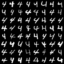
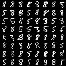
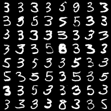
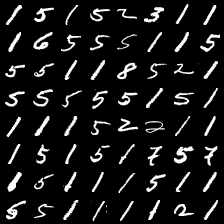
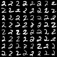
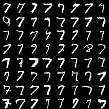
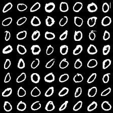
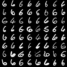
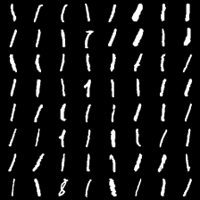
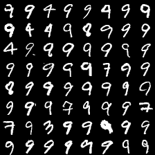
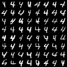
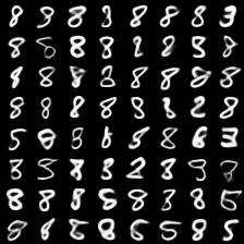
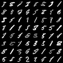
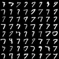
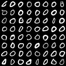
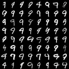
Here are the experimental results for MNIST, including illustrations of samples within classes and sampling by class. Finally, a simple estimation showed that if the most frequent true label in each class is taken as the class label, the final test accuracy is about 83%. Compared to the results in the paper “Unsupervised Deep Embedding for Clustering Analysis” (which also peaks around 84%), this feels quite good.

Clustering Illustration

Sampling by Category

Fashion-MNIST

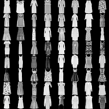
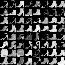
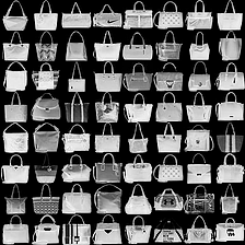
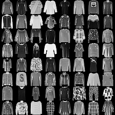
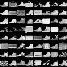
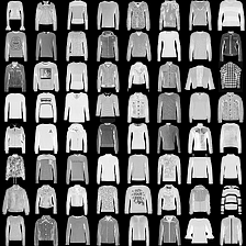
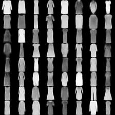
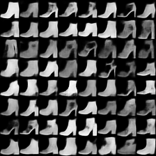
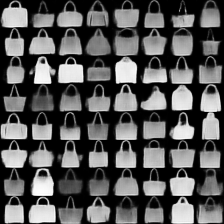
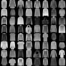
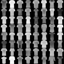
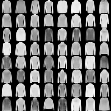
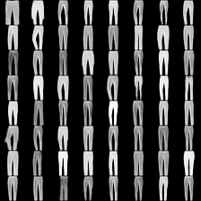
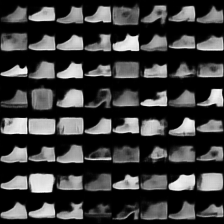
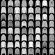
Here are the experimental results for Fashion-MNIST, including illustrations of samples within classes and sampling by class. The final test accuracy is about 58.5%.

Clustering Illustration

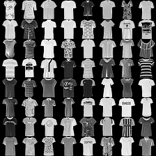
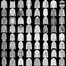
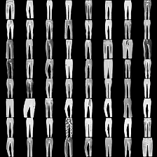
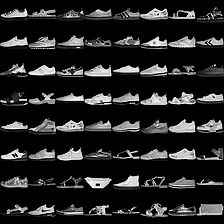
Sampling by Category