Flowing with Flow: RealNVP and Glow—The Inheritance and Sublimation of Flow Models

The Ingenuity of Flow

It must be said that the flow model is a very ingeniously designed model. Overall, flow aims to find an encoder that encodes the input \boldsymbol{x} into a latent variable \boldsymbol{z}, such that \boldsymbol{z} follows a standard normal distribution. Thanks to the clever design of the flow model, this encoder is reversible, allowing us to immediately write down the corresponding decoder (generator). Therefore, as soon as the encoder is trained, we simultaneously obtain the decoder, completing the construction of the generative model.

To realize this concept, the model must not only be reversible but also ensure that the corresponding Jacobian determinant is easy to calculate. To this end, NICE proposed the additive coupling layer. By stacking multiple additive coupling layers, the model possesses both powerful fitting capabilities and a unit Jacobian determinant. Thus, a generative model different from VAE and GAN—the flow model—emerged. Through its clever construction, it allows us to directly fit the probability distribution itself.

Space to Explore

NICE provided a new way of thinking for flow models and completed simple experiments, but it also left much unknown space. While the concept of flow models is ingenious, the experiments in NICE were relatively crude: it simply stacked fully connected layers and did not provide usage for convolutional layers. Although the paper conducted several experiments, the only truly successful one was on MNIST, which lacked sufficient persuasiveness.

Therefore, flow models needed further exploration to become more prominent in the field of generative models. These extensions were completed by its "successors," RealNVP and Glow. Their work made flow models shine, turning them into leaders in the field of generative models.

Affine Coupling Layer

The first author of both NICE and RealNVP is Laurent Dinh, a PhD student of Bengio. His pursuit and refinement of flow models are truly admirable. In the first NICE paper, he proposed the additive coupling layer and actually mentioned the multiplicative coupling layer, though it wasn’t used. In RealNVP, additive and multiplicative coupling layers are combined into a general "affine coupling layer." \begin{aligned} &\boldsymbol{h}_{1} = \boldsymbol{x}_{1}\\ &\boldsymbol{h}_{2} = \boldsymbol{s}(\boldsymbol{x}_{1})\otimes\boldsymbol{x}_{2} + \boldsymbol{t}(\boldsymbol{x}_{1}) \end{aligned} Here, \boldsymbol{s} and \boldsymbol{t} are vector functions of \boldsymbol{x}_1. Formally, the second equation corresponds to an affine transformation of \boldsymbol{x}_2, hence the name "affine coupling layer."

The Jacobian matrix of the affine coupling is still a triangular matrix, but the diagonal is not all 1s. Represented as a block matrix: \left[\frac{\partial \boldsymbol{h}}{\partial \boldsymbol{x}}\right]=\begin{pmatrix}\mathbb{I}_d & \mathbb{O} \\ \left[\frac{\partial \boldsymbol{s}}{\partial \boldsymbol{x}_1}\otimes \boldsymbol{x}_2+\frac{\partial \boldsymbol{t}}{\partial \boldsymbol{x}_1}\right] & \text{diag}(\boldsymbol{s})\end{pmatrix} Clearly, its determinant is the product of the elements of \boldsymbol{s}. To ensure reversibility, we generally constrain the elements of \boldsymbol{s} to be greater than zero. Thus, we usually use a neural network to output \log \boldsymbol{s} and then take the exponential form e^{\log \boldsymbol{s}}.

Note: The name RealNVP likely comes from the affine layer. Its full name is "real-valued non-volume preserving." Compared to the additive coupling layer where the determinant is 1, the Jacobian determinant of RealNVP is no longer constantly equal to 1. Since the geometric meaning of the determinant is volume, a determinant of 1 means the volume remains unchanged, while a determinant not equal to 1 means the volume changes—hence "non-volume preserving."

Random Shuffling of Dimensions

In NICE, the author mixed the information flow through interleaving (which is theoretically equivalent to reversing the original vector), as shown below (correspondingly, the diagram here uses the affine coupling layer):

RealNVP found that shuffling the vector randomly allows information to mix more thoroughly, resulting in a lower final loss:

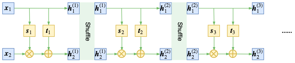
Random shuffling here refers to concatenating the two vectors \boldsymbol{h}_1, \boldsymbol{h}_2 output by each flow step into a single vector \boldsymbol{h} and then re-sorting this vector randomly.

Introducing Convolutional Layers

RealNVP provides a scheme for reasonably using convolutional neural networks in flow models, which allows us to better handle image problems, reduce the number of parameters, and fully utilize the parallel performance of the model.

Note that applying convolution is not reasonable in all cases. The prerequisite for using convolution is that the input has local correlation (in the spatial dimension). Images themselves have local correlation because adjacent pixels are related. However, we must note two operations in flow: 1. Splitting the input into two parts \boldsymbol{x}_1, \boldsymbol{x}_2 and feeding them into the coupling layer, where the models \boldsymbol{s}, \boldsymbol{t} actually only process \boldsymbol{x}_1; 2. Randomly shuffling the dimensions of the features before they enter the coupling layer. Both operations can destroy local correlation. For example, splitting might separate adjacent pixels, and random shuffling might move adjacent pixels far apart.

Therefore, to use convolution, one must find a way to preserve spatial local correlation. We know an image has three axes: height, width, and channel. The first two are spatial axes and clearly have local correlation. Thus, the only axis we can "mess with" is the "channel" axis. To this end, RealNVP stipulates that splitting and shuffling operations are only performed on the "channel" axis. That is, after splitting the input into \boldsymbol{x}_1, \boldsymbol{x}_2 along the channels, \boldsymbol{x}_1 still retains local correlation. Similarly, after shuffling the whole along the channels in the same way, spatial correlation is preserved, allowing the use of convolution in models \boldsymbol{s}, \boldsymbol{t}.

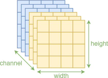
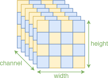
Note: In RealNVP, the operation of splitting the input into two parts is called a mask, as it is equivalent to using 0/1 to label the original input. Besides the channel-wise mask mentioned above, RealNVP also introduced a spatial interleaved mask, as shown on the right above, called a checkerboard mask. This special split also preserves spatial local correlation. The original paper used both mask types alternately, but the checkerboard mask is relatively complex and does not offer a significant improvement, so it was abandoned in Glow.

However, a problem arises. General image channel axes are only three-dimensional, and grayscale images like MNIST have only one. How do you split them in half? How do you shuffle them? To solve this, RealNVP introduced the "squeeze" operation to give the channel axis higher dimensionality. The idea is simple: direct reshaping, but performed locally. Specifically, assume the original image is h \times w \times c. Divide it along the spatial dimensions into 2 \times 2 \times c blocks (the 2 can be customized), and then reshape each block into 1 \times 1 \times 4c. The result is an image of size h/2 \times w/2 \times 4c.

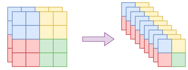
With the squeeze operation, we can increase the dimensionality of the channel axis while preserving local correlation, allowing everything we discussed to proceed. Thus, squeeze has become an essential operation for flow models in image applications.

Multi-scale Structure

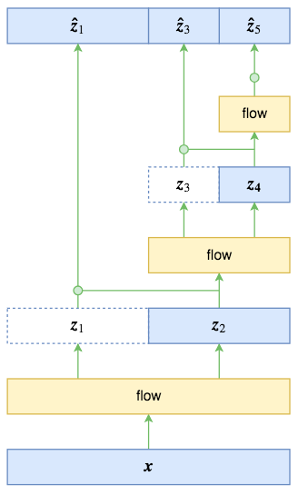
In addition to successfully introducing convolutional layers, another important advancement in RealNVP is the addition of a multi-scale structure. Like convolutional layers, this is a strategy that both reduces model complexity and improves results.

The multi-scale structure is not complex. As shown in the figure, after the original input undergoes the first flow step (a "flow step" refers to the composition of multiple affine coupling layers), the output is the same size as the input. At this point, the input is split into two halves \boldsymbol{z}_1, \boldsymbol{z}_2 (along the channel axis). \boldsymbol{z}_1 is output directly, while only \boldsymbol{z}_2 is sent to the next flow step, and so on. In the specific example in the figure, the final output consists of [\boldsymbol{z}_1, \boldsymbol{z}_3, \boldsymbol{z}_5], with a total size equal to the input.

The multi-scale structure has a "fractal" flavor; the original paper says it was inspired by VGG. Each step of the multi-scale operation directly reduces the data size to half of the previous step, which is quite significant. However, there is an important detail mentioned in neither the RealNVP nor the Glow papers, which I only understood after reading the source code: how should the prior distribution of the final output [\boldsymbol{z}_1, \boldsymbol{z}_3, \boldsymbol{z}_5] be chosen? Following the general assumption of flow models, should it be set directly as a standard normal distribution?

In fact, as multi-scale outputs at different positions, \boldsymbol{z}_1, \boldsymbol{z}_3, \boldsymbol{z}_5 do not have equal status. Simply setting a global standard normal distribution would force them to be equivalent, which is unreasonable. The best approach is to write out the conditional probability formula: p(\boldsymbol{z}_1, \boldsymbol{z}_3, \boldsymbol{z}_5) = p(\boldsymbol{z}_1|\boldsymbol{z}_3, \boldsymbol{z}_5)p(\boldsymbol{z}_3|\boldsymbol{z}_5)p(\boldsymbol{z}_5) Since \boldsymbol{z}_3, \boldsymbol{z}_5 are completely determined by \boldsymbol{z}_2, and \boldsymbol{z}_5 is completely determined by \boldsymbol{z}_4, the conditional part can be changed to: p(\boldsymbol{z}_1, \boldsymbol{z}_3, \boldsymbol{z}_5) = p(\boldsymbol{z}_1|\boldsymbol{z}_2)p(\boldsymbol{z}_3|\boldsymbol{z}_4)p(\boldsymbol{z}_5) RealNVP and Glow assume that the three probability distributions on the right are all normal distributions, where the mean and variance of p(\boldsymbol{z}_1|\boldsymbol{z}_2) are calculated from \boldsymbol{z}_2 (e.g., via convolution, similar to VAE), the mean and variance of p(\boldsymbol{z}_3|\boldsymbol{z}_4) are calculated from \boldsymbol{z}_4, and the mean and variance of p(\boldsymbol{z}_5) are learned directly.

Clearly, this assumption is much more effective than simply assuming they are all standard normal. We can also express this differently: the above prior assumption is equivalent to the following variable substitution: \boldsymbol{\hat{z}}_1 = \frac{\boldsymbol{z}_1 - \boldsymbol{\mu}(\boldsymbol{z}_2)}{\boldsymbol{\sigma}(\boldsymbol{z}_2)}, \quad \boldsymbol{\hat{z}}_3 = \frac{\boldsymbol{z}_3 - \boldsymbol{\mu}(\boldsymbol{z}_4)}{\boldsymbol{\sigma}(\boldsymbol{z}_4)}, \quad \boldsymbol{\hat{z}}_5 = \frac{\boldsymbol{z}_5 - \boldsymbol{\mu}}{\boldsymbol{\sigma}} And then assuming [\boldsymbol{\hat{z}}_1, \boldsymbol{\hat{z}}_3, \boldsymbol{\hat{z}}_5] follows a standard normal distribution. Like the scale transformation layer in NICE, these three transformations result in a non-unit Jacobian determinant, which means adding a term like \sum_{i=1}^D \log \boldsymbol{\sigma}_i to the loss.

At first glance, the multi-scale structure seems to be for reducing computation, but it is not that simple. Due to the reversibility of flow models, the input and output dimensions are the same, which actually leads to a serious dimension waste problem. This often requires us to use sufficiently complex networks to mitigate it. The multi-scale structure is equivalent to abandoning the direct assumption that p(\boldsymbol{z}) is a standard normal distribution and instead adopting a composite conditional distribution. Thus, although the total input and output dimensions remain the same, the status of outputs at different levels is no longer equal. The model can suppress the dimension waste problem by controlling the variance of each conditional distribution (in the extreme case, if the variance is 0, the Gaussian collapses to a Dirac distribution, reducing the dimension by 1). Conditional distributions offer greater flexibility than independent ones. From the perspective of loss, the multi-scale structure provides a powerful regularization term (equivalent to multiple shortcut connections in a multi-layer image classification model).

Invertible 1 \times 1 Convolution

This section introduces the main improvement of Glow: the invertible 1 \times 1 convolution.

Results Analysis

The above description is based on fully connected layers. If applied to images, the same operation is performed on each channel vector, which is equivalent to a 1 \times 1 convolution. This is the origin of the so-called invertible 1 \times 1 convolution. In fact, I think the name is not quite ideal; it is essentially a weight-sharing, invertible fully connected layer. Calling it a 1 \times 1 convolution limits it to images, which is not general enough.

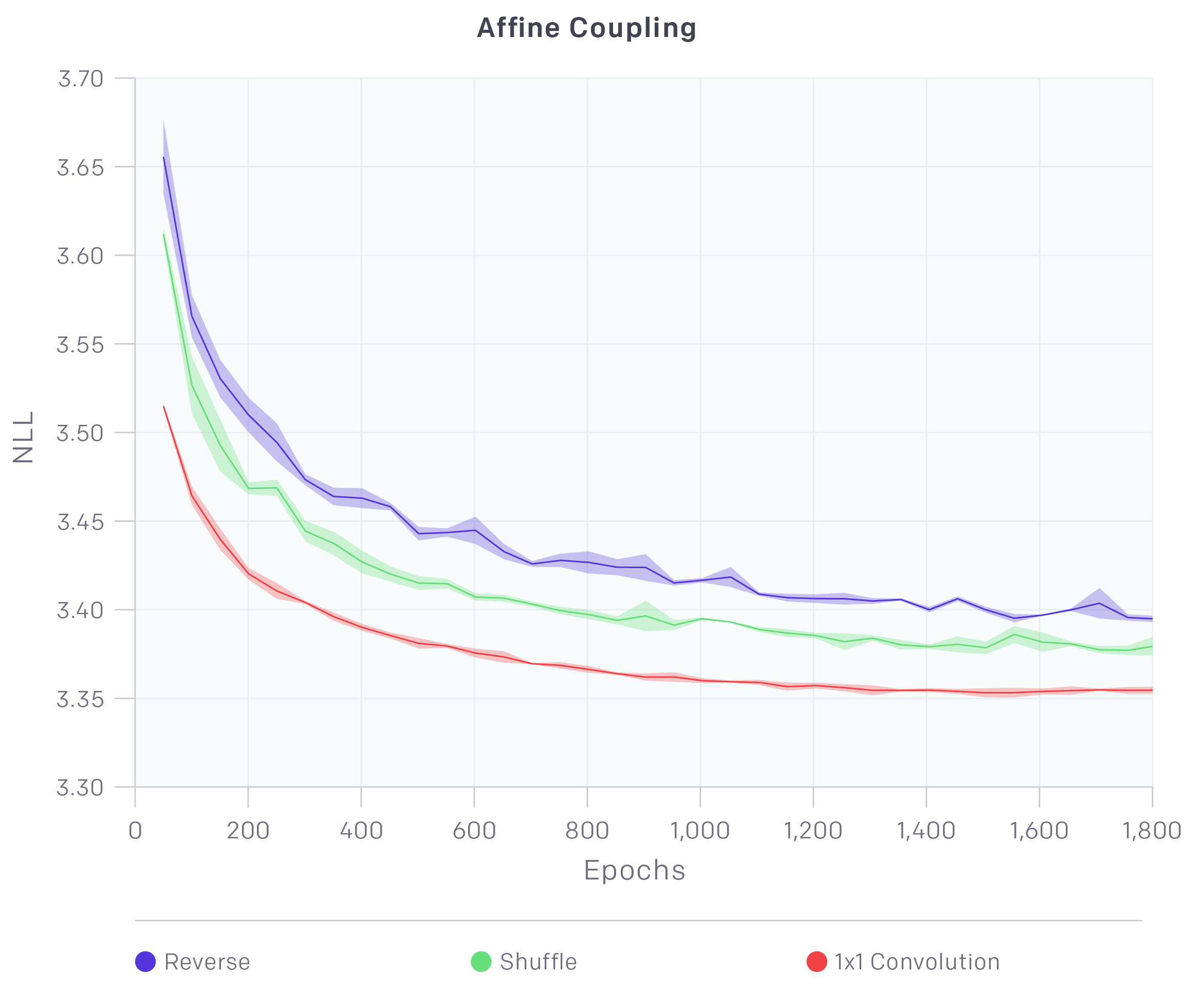
The Glow paper conducted comparative experiments showing that compared to simple reversal, shuffle achieves a lower loss, and compared to shuffle, invertible 1 \times 1 convolution achieves an even lower loss. My own experiments confirm this.

However, it should be noted: while invertible 1 \times 1 convolution reduces loss, there are issues to consider. First, a lower loss does not necessarily mean higher generation quality. For example, if model A uses shuffle and reaches loss = -50,000 after 200 epochs, and model B uses invertible convolution and reaches loss = -55,000 after 150 epochs, usually model B’s effect is not as good as A’s in the current state (assuming neither has reached the optimum). Invertible 1 \times 1 convolution only guarantees that if everyone is trained to the optimum, model B will be better. Second, in my own simple experiments, it seems that the number of epochs required for invertible 1 \times 1 convolution to reach saturation is much higher than for simple shuffle.

Actnorm

RealNVP used BN (Batch Normalization) layers, while Glow proposed a layer called Actnorm to replace BN. However, the so-called Actnorm layer is actually just a generalization of the scale transformation layer in NICE, which is the scaling and shifting transformation mentioned in Eq. (5): \boldsymbol{\hat{z}} = \frac{\boldsymbol{z} - \boldsymbol{\mu}}{\boldsymbol{\sigma}} where \boldsymbol{\mu}, \boldsymbol{\sigma} are trainable parameters. Glow’s innovation in the paper was to use the mean and variance of the initial batch to initialize \boldsymbol{\mu}, \boldsymbol{\sigma}, but the provided source code does not actually do this; it uses zero initialization.

Therefore, this point deserves criticism—it’s simply giving an old concept a new name. Of course, the criticism is directed at OpenAI for creating new terms in Glow, not at the effect of the layer. The addition of scaling and shifting indeed helps in training the model better. Moreover, due to the existence of Actnorm, the scale transformation in the affine coupling layer has become less important. We see that compared to the additive coupling layer, the affine coupling layer has an extra scale transformation, doubling the computation. But in fact, compared to additive coupling, the improvement of affine coupling is not high (especially after adding Actnorm). So to train large models and save resources, generally only additive coupling is used. For example, Glow used only additive coupling to train the 256 \times 256 high-definition face generation model.

Source Code Analysis

In fact, there isn’t much more to interpret about Glow. However, the overall Glow model is quite standardized. We can decompose the structure of the Glow model step by step to provide a reference for building similar models. This part comes from my reading of the Glow source code and is presented mainly through diagrams.

Overall Model Diagram

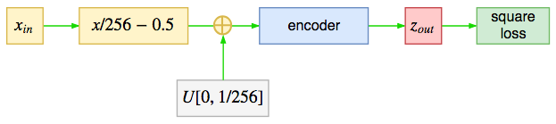
Overall, the Glow model is not complex. It adds a certain amount of noise to the input, feeds it into an encoder, and finally uses the "average sum of squares of the output" as the loss function (the log-Jacobian determinant generated in the model can be seen as a regularization term). Note that the loss is not "Mean Squared Error (MSE)," but simply the sum of squares of the output—meaning you don’t subtract the input.

Encoder

Decomposing the encoder from the overall diagram, the process is roughly:

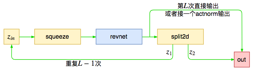
The encoder consists of L modules, named "revnet" in the source code. Each module operates on the input and then splits the output into two halves: one half goes to the next module, and the other half is output directly. This is the multi-scale structure mentioned earlier. Glow defaults to L=3, but for 256 \times 256 face generation, L=6 is used.

revnet

Now let’s further decompose the revnet part:

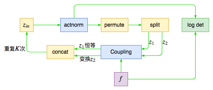
It is essentially the single-step flow operation described earlier: scale transformation before input, axis shuffling, splitting, and then feeding into the coupling layer. This is trained K times, where K is called the "depth," defaulting to 32 in Glow. Actnorm and the affine coupling layer bring non-unit Jacobian determinants, which modify the loss, as noted in the diagram.

split2d

The split2d defined in Glow is not a simple split but a mixture of transformation operations after splitting, which is the prior distribution selection for multi-scale outputs mentioned earlier.

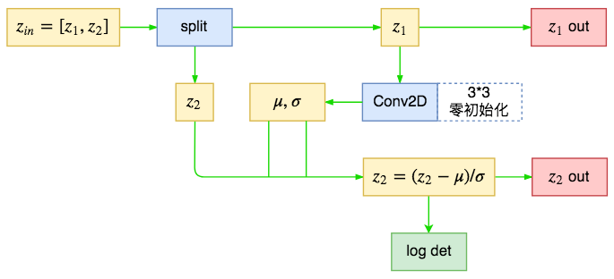
Comparing Eq. (5) and Eq. (10), we find that the difference between the conditional prior distribution and Actnorm is only the source of the scaling and shifting amounts. In Actnorm, they are optimized directly, while in the prior distribution, they are calculated from another part through some model. In fact, we can consider this a form of Conditional Actnorm (Cond Actnorm).

f

Finally, the model for the coupling layer in Glow (the \boldsymbol{s}, \boldsymbol{t} of the affine coupling layer) is named "f" in the source code. It uses three layers of ReLU convolutions:

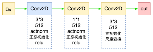
The last layer uses zero initialization, so the initial state of the input and output is the same—an identity transformation—which helps in training deep networks.

Keras Version

The officially open-sourced Glow is in TensorFlow. For such an interesting model, how could there not be a Keras version? Here is the Keras version I implemented:
https://github.com/bojone/flow/blob/master/glow.py
(I have submitted a pull request to the official Keras examples; hopefully, it will be on Keras’s GitHub in a few days.)

Due to certain function limitations, it currently only supports the TensorFlow backend. My testing environment includes: Keras 2.1.5 + TensorFlow 1.2 and Keras 2.2.0 + TensorFlow 1.8, both tested under Python 2.7.

Effectiveness Testing

When I first read about Glow, I was very excited, as if I had discovered a new continent. After some study, I found... Glow is indeed a new continent, but not one that commoners like us can easily set foot on.

Let’s look at two issues on Glow’s GitHub:

"How many epochs will be take when training celeba?"
The samples we show in the paper are after about 4000 training epochs...

"anyone reproduced the celeba-HQ results in the paper"
Yes we trained with 40 GPU’s for about a week, but samples did start to look good after a couple of days...

We see that 256 \times 256 high-definition face generation requires training for 4000 epochs, using 40 GPUs for a week. Simply put, that’s like training for a year on one GPU... (Dead).

Well, I’ll give up on that unreachable task. Let’s just play with 64 \times 64, or rather, 32 \times 32 face generation and make a demo.

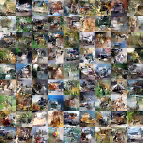
It looks okay. I used L=3, K=6, and each epoch took about 70s (GTX 1070). I ran it for 150 epochs. The "epoch" here is different from the usual concept; one epoch for me is 32,000 randomly sampled instances. If I ran a full epoch every time, it would take much longer... I also ran CIFAR-10 with the same model for 700 epochs, but the effect wasn’t great. It looks okay from afar, but up close, it’s nothing.

Of course, although CIFAR-10 is small (32 \times 32), generating CIFAR-10 is actually much harder than generating faces (for any generative model), so let’s skip that. As for 64 \times 64 faces, I recklessly tried it with L=3, K=10, running for 200 epochs (each epoch took 6 minutes). The result...

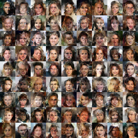
They are faces, but they look more like demon faces... (It seems the network depth and number of epochs are not enough, and I can’t keep running it).

The temperature parameter is also quite important. After changing the temperature parameter to 0.8, the same model’s generation result is:

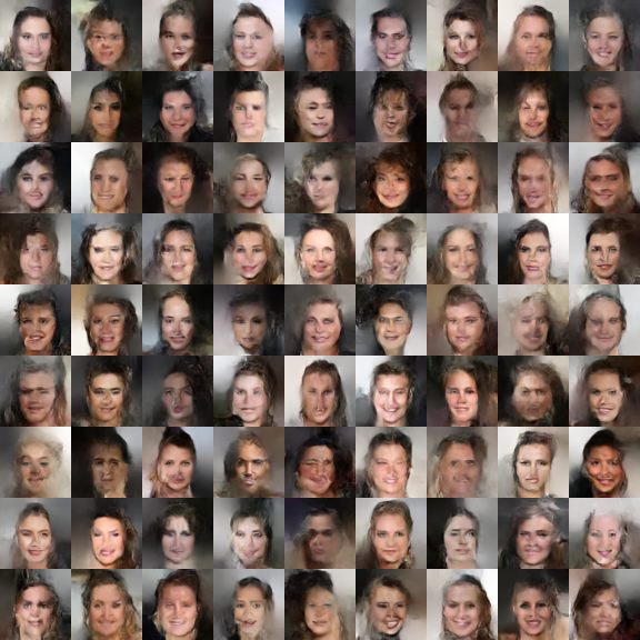
Still a bit distorted, but it looks much better.