NICE: Basic Concepts and Implementation of Flow Models

The Difficulty of Distributions

As is well known, the current mainstream generative models include VAEs and GANs. However, in addition to these two, there are also models based on "flow." In fact, the history of flow is as long as that of VAEs and GANs, yet flow remains relatively obscure. In my view, the likely reason is that flow lacks an intuitive explanation like the "counterfeiter-discriminator" analogy of GANs. Flow is inherently more mathematical, and its early results were not particularly good while being computationally expensive, making it hard to generate interest. However, it now seems that OpenAI’s stunning Glow model will likely encourage more people to invest in improving flow models.

The essence of a generative model is the hope of using a known probability model to fit given data samples. That is, we must write a distribution q_{\boldsymbol{\theta}}(\boldsymbol{x}) with parameters \boldsymbol{\theta}. However, our neural networks are "universal function approximators," not "universal distribution approximators." While they can, in principle, fit any function, they cannot arbitrarily fit a probability distribution because distributions must satisfy "non-negativity" and "normalization" requirements. Consequently, the only distributions we can write directly are discrete distributions or continuous Gaussian distributions.

Of course, from a strict perspective, an image should be a discrete distribution because it consists of a finite number of pixels, and each pixel value is discrete and finite. Thus, it can be described by a discrete distribution. The result of this line of thought is models like PixelRNN, which we call "autoregressive flows." Their characteristic is that they cannot be parallelized, leading to extremely high computational costs. Therefore, we prefer to use continuous distributions to describe images. Images are just one scenario; we have many other types of continuous data, making the study of continuous distributions essential.

Different Approaches

The problem arises: for continuous data, we can essentially only write down Gaussian distributions. Furthermore, for ease of processing, we often only write Gaussians with independent components. This is clearly a tiny fraction of all continuous distributions and is insufficient. To solve this dilemma, we create more distributions through integration: q(\boldsymbol{x})=\int q(\boldsymbol{z})q_{\boldsymbol{\theta}}(\boldsymbol{x}|\boldsymbol{z}) d\boldsymbol{z}\tag{1} Here q(\boldsymbol{z}) is typically a standard Gaussian distribution, and q_{\boldsymbol{\theta}}(\boldsymbol{x}|\boldsymbol{z}) can be any conditional Gaussian or Dirac delta distribution. This integral form can create many complex distributions. Theoretically, it can fit any distribution.

Now that we have the distribution form, we need to find the parameters \boldsymbol{\theta}, usually via maximum likelihood. Assuming the true data distribution is \tilde{p}(\boldsymbol{x}), we need to maximize: \mathbb{E}_{\boldsymbol{x}\sim \tilde{p}(\boldsymbol{x})} \big[\log q(\boldsymbol{x})\big]\tag{2} However, since q_{\boldsymbol{\theta}}(\boldsymbol{x}) is in integral form, whether it can be computed is uncertain.

Various experts have used different methods to bypass this difficulty. VAEs do not directly optimize objective (2) but instead optimize a tighter upper bound, which makes them approximate models that may struggle to achieve perfect generation. GANs bypass the difficulty through an alternating training method, preserving the model’s precision, which is why they achieve such good results. Nevertheless, GANs are not perfect in every aspect, so exploring other solutions is meaningful.

Facing the Probability Integral Directly

Flow models choose a "hard path": calculating the integral directly.

Specifically, flow models choose q(\boldsymbol{x}|\boldsymbol{z}) to be the Dirac distribution \delta(\boldsymbol{x}-\boldsymbol{g}(\boldsymbol{z})), where \boldsymbol{g}(\boldsymbol{z}) must be reversible. That is: \boldsymbol{x}=\boldsymbol{g}(\boldsymbol{z}) \Leftrightarrow \boldsymbol{z} = \boldsymbol{f}(\boldsymbol{x})\tag{3} To achieve reversibility theoretically (mathematically), \boldsymbol{z} and \boldsymbol{x} must have the same dimension. Assuming the forms of \boldsymbol{f} and \boldsymbol{g} are known, calculating q(\boldsymbol{x}) via (1) is equivalent to performing an integral transformation \boldsymbol{z}=\boldsymbol{f}(\boldsymbol{x}) on q(\boldsymbol{z}). That is, starting from: q(\boldsymbol{z}) = \frac{1}{(2\pi)^{D/2}}\exp\left(-\frac{1}{2} \Vert \boldsymbol{z}\Vert^2\right)\tag{4} which is a standard Gaussian distribution (D is the dimension of \boldsymbol{z}), we apply the transformation \boldsymbol{z}=\boldsymbol{f}(\boldsymbol{x}). Note that the change of variables for a probability density function is not simply replacing \boldsymbol{z} with \boldsymbol{f}(\boldsymbol{x}); it also introduces the absolute value of the "Jacobian determinant": q(\boldsymbol{x}) = \frac{1}{(2\pi)^{D/2}}\exp\left(-\frac{1}{2}\big\Vert \boldsymbol{f}(\boldsymbol{x})\big\Vert^2\right)\left|\det\left[\frac{\partial \boldsymbol{f}}{\partial \boldsymbol{x}}\right]\right|\tag{5} Thus, we have two requirements for \boldsymbol{f}:

1. It must be reversible, and the inverse function must be easy to find (its inverse \boldsymbol{g} is our desired generative model);
2. The corresponding Jacobian determinant must be easy to calculate.

Consequently: \log q(\boldsymbol{x}) = -\frac{D}{2}\log (2\pi) -\frac{1}{2}\big\Vert \boldsymbol{f}(\boldsymbol{x})\big\Vert^2 + \log \left|\det\left[\frac{\partial \boldsymbol{f}}{\partial \boldsymbol{x}}\right]\right|\tag{6} This optimization objective is solvable. Furthermore, since \boldsymbol{f} is easy to invert, once training is complete, we can randomly sample \boldsymbol{z} and generate a sample via the inverse of \boldsymbol{f}: \boldsymbol{f}^{-1}(\boldsymbol{z})=\boldsymbol{g}(\boldsymbol{z}). This gives us the generative model.

Block Coupling Layers

Relatively speaking, calculating the determinant is more difficult than inverting a function, so we start from "Requirement 2." Those familiar with linear algebra know that the determinant of a triangular matrix is the easiest to calculate: it is the product of the diagonal elements. Therefore, we should find a way to make the Jacobian matrix of the transformation \boldsymbol{f} triangular. NICE uses a clever approach: it divides the D-dimensional \boldsymbol{x} into two parts \boldsymbol{x}_1, \boldsymbol{x}_2, and applies the following transformation: \begin{aligned} &\boldsymbol{h}_{1} = \boldsymbol{x}_{1}\\ &\boldsymbol{h}_{2} = \boldsymbol{x}_{2} + \boldsymbol{m}(\boldsymbol{x}_{1}) \end{aligned}\tag{7} where \boldsymbol{x}_1, \boldsymbol{x}_2 is a partition of \boldsymbol{x}, and \boldsymbol{m} is an arbitrary function of \boldsymbol{x}_1. That is, \boldsymbol{x} is split, and the transformation is applied to obtain a new variable \boldsymbol{h}. we call this an "Additive Coupling Layer". Without loss of generality, the dimensions of \boldsymbol{x} can be rearranged such that \boldsymbol{x}_1 = \boldsymbol{x}_{1:d} are the first d elements and \boldsymbol{x}_2 = \boldsymbol{x}_{d+1:D} are the remaining elements.

It is easy to see that the Jacobian matrix \left[\frac{\partial \boldsymbol{h}}{\partial \boldsymbol{x}}\right] of this transformation is a triangular matrix with 1s on the diagonal. In block matrix form: \left[\frac{\partial \boldsymbol{h}}{\partial \boldsymbol{x}}\right]=\begin{pmatrix}\mathbb{I}_{1:d} & \mathbb{O} \\ \left[\frac{\partial \boldsymbol{m}}{\partial \boldsymbol{x}_1}\right] & \mathbb{I}_{d+1:D}\end{pmatrix}\tag{8} Thus, the Jacobian determinant of this transformation is 1, and its logarithm is 0, solving the determinant calculation problem.

At the same time, the transformation in (7) is reversible, with the inverse: \begin{aligned} &\boldsymbol{x}_{1} = \boldsymbol{h}_{1}\\ &\boldsymbol{x}_{2} = \boldsymbol{h}_{2} - \boldsymbol{m}(\boldsymbol{h}_{1}) \end{aligned}\tag{9}

The Steady Stream of Flow

The above transformation is surprising: it is reversible, and the inverse is simple, adding no extra computational cost. However, we notice that the first part of transformation (7) is trivial (an identity transformation). Thus, a single transformation cannot achieve strong non-linearity. We need to compose multiple simple transformations to achieve strong non-linearity and enhance fitting capability: \boldsymbol{x} = \boldsymbol{h}^{(0)} \leftrightarrow \boldsymbol{h}^{(1)} \leftrightarrow \boldsymbol{h}^{(2)} \leftrightarrow \dots \leftrightarrow \boldsymbol{h}^{(n-1)} \leftrightarrow \boldsymbol{h}^{(n)} = \boldsymbol{z}\tag{10} Each transformation is an additive coupling layer. This is like a stream of water—accumulating bit by bit—hence the term "flow." In other words, a flow is the coupling of multiple additive coupling layers.

By the chain rule: \left[\frac{\partial \boldsymbol{z}}{\partial \boldsymbol{x}}\right]=\left[\frac{\partial \boldsymbol{h}^{(n)}}{\partial \boldsymbol{h}^{(0)}}\right]=\left[\frac{\partial \boldsymbol{h}^{(n)}}{\partial \boldsymbol{h}^{(n-1)}}\right]\left[\frac{\partial \boldsymbol{h}^{(n-1)}}{\partial \boldsymbol{h}^{(n-2)}}\right]\dots \left[\frac{\partial \boldsymbol{h}^{(1)}}{\partial \boldsymbol{h}^{(0)}}\right]\tag{11} Since "the determinant of a product of matrices equals the product of the determinants," and each layer is an additive coupling layer with a determinant of 1, the result is: \det \left[\frac{\partial \boldsymbol{z}}{\partial \boldsymbol{x}}\right]=\det\left[\frac{\partial \boldsymbol{h}^{(n)}}{\partial \boldsymbol{h}^{(n-1)}}\right]\det\left[\frac{\partial \boldsymbol{h}^{(n-1)}}{\partial \boldsymbol{h}^{(n-2)}}\right]\dots \det\left[\frac{\partial \boldsymbol{h}^{(1)}}{\partial \boldsymbol{h}^{(0)}}\right]=1 (Considering the staggering below, the determinant might become -1, but the absolute value remains 1), so we still do not need to worry about the determinant.

Advancing Through Interleaving

Note that if the coupling order remains unchanged, i.e.: \begin{array}{ll} \begin{aligned} &\boldsymbol{h}^{(1)}_{1} = \boldsymbol{x}_{1}\\ &\boldsymbol{h}^{(1)}_{2} = \boldsymbol{x}_{2} + \boldsymbol{m}_1(\boldsymbol{x}_{1}) \end{aligned} & \begin{aligned} &\boldsymbol{h}^{(2)}_{1} = \boldsymbol{h}^{(1)}_{1}\\ &\boldsymbol{h}^{(2)}_{2} = \boldsymbol{h}^{(1)}_{2} + \boldsymbol{m}_2\big(\boldsymbol{h}^{(1)}_{1}\big) \end{aligned} \\ & \\ \begin{aligned} &\boldsymbol{h}^{(3)}_{1} = \boldsymbol{h}^{(2)}_{1}\\ &\boldsymbol{h}^{(3)}_{2} = \boldsymbol{h}^{(2)}_{2} + \boldsymbol{m}_3\big(\boldsymbol{h}^{(2)}_{1}\big) \end{aligned} & \begin{aligned} &\boldsymbol{h}^{(4)}_{1} = \boldsymbol{h}^{(3)}_{1}\\ &\boldsymbol{h}^{(4)}_{2} = \boldsymbol{h}^{(3)}_{2} + \boldsymbol{m}_4\big(\boldsymbol{h}^{(3)}_{1}\big) \end{aligned} \quad\dots \end{array}\tag{12} Then \boldsymbol{z}_1 = \boldsymbol{x}_1 will still hold, and the first part remains trivial, as shown below:

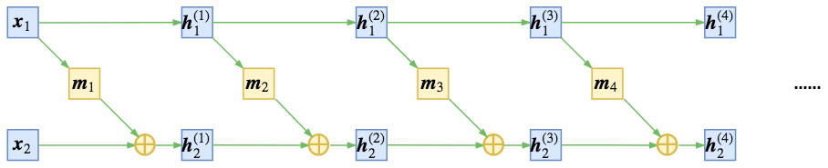
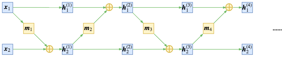
To obtain a non-trivial transformation, we can consider shuffling or reversing the order of the input dimensions before each additive coupling, or simply swapping the positions of the two parts so that information can be fully mixed: \begin{array}{ll} \begin{aligned} &\boldsymbol{h}^{(1)}_{1} = \boldsymbol{x}_{1}\\ &\boldsymbol{h}^{(1)}_{2} = \boldsymbol{x}_{2} + \boldsymbol{m}_1(\boldsymbol{x}_{1}) \end{aligned} & \begin{aligned} &\boldsymbol{h}^{(2)}_{1} = \boldsymbol{h}^{(1)}_{1} + \boldsymbol{m}_2\big(\boldsymbol{h}^{(1)}_{2}\big)\\ &\boldsymbol{h}^{(2)}_{2} = \boldsymbol{h}^{(1)}_{2} \end{aligned} \\ & \\ \begin{aligned} &\boldsymbol{h}^{(3)}_{1} = \boldsymbol{h}^{(2)}_{1}\\ &\boldsymbol{h}^{(3)}_{2} = \boldsymbol{h}^{(2)}_{2} + \boldsymbol{m}_3\big(\boldsymbol{h}^{(2)}_{1}\big) \end{aligned} & \begin{aligned} &\boldsymbol{h}^{(4)}_{1} = \boldsymbol{h}^{(3)}_{1} + \boldsymbol{m}_4\big(\boldsymbol{h}^{(3)}_{2}\big)\\ &\boldsymbol{h}^{(4)}_{2} = \boldsymbol{h}^{(3)}_{2} \end{aligned} \quad\dots \end{array}\tag{13} As shown below:

Scaling Layer

As pointed out earlier, flow is based on reversible transformations. Thus, when the model is trained, we simultaneously obtain a generative model and an encoding model. However, because of the reversible transformation, the random variable \boldsymbol{z} and the input sample \boldsymbol{x} have the same size. When we specify \boldsymbol{z} to follow a Gaussian distribution, it spans the entire D-dimensional space, where D is the size of the input \boldsymbol{x}. But while \boldsymbol{x} has D dimensions, it might not actually span the entire D-dimensional space. For example, although an MNIST image has 784 pixels, some pixels remain 0 in both the training and test sets, indicating the data manifold is much smaller than 784 dimensions.

In other words, flow models based on reversible transformations naturally suffer from a serious "dimension waste" problem: the input data is clearly not a D-dimensional manifold, yet it must be encoded as one. Is this feasible?

To address this, NICE introduces a scaling layer. it applies a scale transformation to each dimension of the final encoded features, i.e., \boldsymbol{z} = \boldsymbol{s}\otimes \boldsymbol{h}^{(n)}, where \boldsymbol{s} = (\boldsymbol{s}_1,\boldsymbol{s}_2,\dots,\boldsymbol{s}_D) is a parameter vector to be optimized (with non-negative elements). This \boldsymbol{s} vector can identify the importance of each dimension (smaller values are more important; larger values indicate the dimension is less important and nearly negligible), acting to compress the manifold. Note that the Jacobian determinant of this scaling layer is no longer 1; its Jacobian matrix is diagonal: \left[\frac{\partial \boldsymbol{z}}{\partial \boldsymbol{h}^{(n)}}\right] = \text{diag}\, (\boldsymbol{s})\tag{14} So its determinant is \prod_i \boldsymbol{s}_i. According to equation (6), the log-likelihood is: \log q(\boldsymbol{x}) \sim -\frac{1}{2}\big\Vert \boldsymbol{s}\otimes \boldsymbol{f} (\boldsymbol{x})\big\Vert^2 + \sum_i \log \boldsymbol{s}_i\tag{15}

Why can this scaling identify feature importance? In fact, the scaling layer can be described in a clearer way: we initially set the prior distribution of \boldsymbol{z} to be a standard normal distribution (variance of 1). In fact, we can treat the variance of the prior distribution as a trainable parameter. After training, the variances will vary. A smaller variance means the "dispersion" of that feature is smaller. If the variance were 0, the feature would always be the mean 0, and the distribution of that dimension would collapse to a point, meaning the manifold dimension is reduced by one.

Unlike equation (4), we write the normal distribution with variance: q(\boldsymbol{z}) = \frac{1}{(2\pi)^{D/2}\prod\limits_{i=1}^D \boldsymbol{\sigma}_i}\exp\left(-\frac{1}{2}\sum_{i=1}^D \frac{\boldsymbol{z}_i^2}{\boldsymbol{\sigma}_i^2}\right)\tag{16} Substituting the flow model \boldsymbol{z}=\boldsymbol{f}(\boldsymbol{x}) into the above and taking the logarithm, similar to (6), we get: \log q(\boldsymbol{x}) \sim -\frac{1}{2}\sum_{i=1}^D \frac{\boldsymbol{f}_i^2(\boldsymbol{x})}{\boldsymbol{\sigma}_i^2} - \sum_{i=1}^D \log \boldsymbol{\sigma}_i\tag{17} Comparing with (15), we have \boldsymbol{s}_i=1/\boldsymbol{\sigma}_i. Thus, the scaling layer is equivalent to treating the prior distribution’s variance (standard deviation) as a trainable parameter. If the variance is small enough, we can consider the manifold represented by that dimension to have collapsed to a point, thereby reducing the overall manifold dimension by 1, implying the possibility of dimensionality reduction.

Feature Decoupling

When we choose the prior distribution to be a Gaussian with independent components, what benefits does it bring besides sampling convenience?

In a flow model, \boldsymbol{f}^{-1} is the generative model, and \boldsymbol{f} is the encoder. But unlike autoencoders in ordinary neural networks that "force low-dimensional reconstruction of high-dimensional data to extract effective information," flow models are completely reversible, so there is no information loss. What then is the value of this encoder?

This involves the question of "what is a good feature." In reality, we often abstract dimensions to describe things, such as "tall/short," "fat/thin," "beautiful/ugly," "rich/poor." The characteristic of these dimensions is: "When we say someone is tall, they are not necessarily fat or thin, nor are they necessarily rich or poor." That is, there is little necessary connection between these features; otherwise, they would be redundant. Therefore, in an ideal case, the dimensions of a good feature should be independent of each other, achieving feature decoupling so that each dimension has its own independent meaning.

Thus, we can understand the benefit of "a prior distribution with independent Gaussian components." Due to the independence of the components, we can say that when we use \boldsymbol{f} to encode original features, the dimensions of the output encoded features \boldsymbol{z}=\boldsymbol{f}(\boldsymbol{x}) are decoupled. The full name of NICE, "Non-linear Independent Components Estimation," reflects this meaning. Conversely, due to the independence of each dimension of \boldsymbol{z}, we can theoretically change a single dimension to see how the generated image changes, thereby discovering the meaning of that dimension.

Similarly, we can interpolate (weighted average) the encodings of two images to obtain naturally transitioning generated samples. This is fully demonstrated in the later Glow model. However, since we only performed MNIST experiments here, this point is not particularly emphasized in this article.

Model Details

Let’s summarize the parts of the NICE model. NICE is a type of flow model consisting of multiple additive coupling layers. Each layer follows (7), and its inverse is (9). Before coupling, the input dimensions are reversed to ensure information is fully mixed. A scaling layer is added at the end, and the final loss is the negative of (15).

The additive coupling layer needs to split the input into two parts. NICE uses an interleaved partition: even indices for the first part and odd indices for the second. Each \boldsymbol{m}(\boldsymbol{x}) is a simple multi-layer fully connected network (5 hidden layers, 1000 nodes each, ReLU activation). In NICE, a total of 4 additive coupling layers are used.

For the input, we compress the original 0-255 pixel values to the 0-1 range (dividing by 255) and add uniform noise in the range [-0.01, 0]. Adding noise effectively prevents overfitting and improves the quality of generated images. It can also be seen as a measure to alleviate the dimension waste problem, as MNIST images cannot actually fill 784 dimensions, but adding noise increases the dimensionality.

Readers might wonder why the noise interval is [-0.01, 0] instead of [0, 0.01] or [-0.005, 0.005]. In fact, from the perspective of the loss, various types of noise are similar (including replacing uniform noise with Gaussian noise). However, after adding noise, the generated images will theoretically also contain noise. Adding negative noise makes the final generated pixel values slightly biased toward the negative range, allowing us to remove some noise using a clip operation. This is just a small (not particularly critical) trick for MNIST.

Reference Code

Here is my reference implementation using Keras:
https://github.com/bojone/flow/blob/master/nice.py
In my experiments, the model reaches optimality within 20 epochs, taking about 11s per epoch (GTX 1070 environment), with a final loss of approximately -2200.

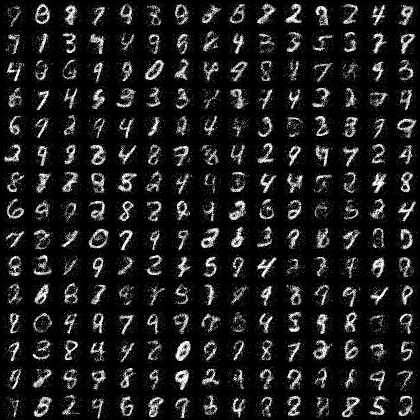
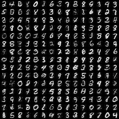
Compared to the original paper’s implementation, some changes were made. For the additive coupling layer, I used (9) for the forward pass and (7) for the inverse. Since \boldsymbol{m}(\boldsymbol{x}) uses ReLU activation, which is non-negative, there is a difference between the two choices. Since the forward pass is the encoder and the inverse is the generator, choosing (7) for the inverse makes the generative model more likely to produce positive numbers, which matches the 0-1 pixel values of the images we want to generate.

Annealing Parameters

Although we ultimately hope to sample random numbers from a standard normal distribution to generate samples, in practice, for a trained model, the ideal sampling variance is not necessarily 1 but fluctuates around 1, generally slightly smaller. The standard deviation of the normal distribution used for final sampling is called the annealing parameter. For example, in the reference implementation above, we chose an annealing parameter of 0.75, which visually yields the best quality from the generative model.