Preface
GAN, which stands for Generative Adversarial Nets, is commonly explained using the "forger-discriminator" analogy, much like a forger and a discriminator of art paintings. Initially, both the forger and the discriminator have low skill levels, but the discriminator can still easily identify the forger’s fakes. As the forger learns better techniques, their fakes begin to deceive the discriminator; conversely, as the discriminator improves, they can easily spot the forger’s work again. This is a process where both parties continuously learn to reach the highest levels of forgery and discrimination. However, readers who look a bit deeper will find that, unlike real-world counterfeiters who use new materials and technologies to keep up with the times, the most magical and confusing part of GAN is its ability to map random noise into the positive samples we desire. With just noise, you get positive samples—isn’t this a business with no capital? How lucrative!
Another observation is that since the introduction of WGAN, mainstream research on GANs has essentially shifted towards WGAN. However, the form of WGAN is actually quite far removed from the "forger-discriminator" explanation. Furthermore, while the final form of WGAN is not complex, its derivation involves a lot of sophisticated mathematics, which discouraged me from studying the original paper. This forced me to find a simple and intuitive path to understand GANs. Fortunately, after some reflection, I have made some progress.
Before we begin, a disclaimer: All my knowledge of GANs comes solely from popular science articles on the internet; I have not directly read any original papers on GANs. Therefore, the results in this article may overlap with mainstream findings or differ significantly, and the narrative method does not follow the historical development of GANs. Rigorous scholars, enter with caution!
Note: Unless otherwise specified, the GANs discussed in this article are in the broad sense, including the original GAN, WGAN, etc., without distinction. Terms like "positive samples" or "real samples" refer to a pre-specified set of samples, while "generated samples" refer to the results obtained by transforming random noise through a generative model G.
An Interview Question
A classic interview question is: If there is a pseudo-random number program that can generate uniform random numbers between [0,1], how can it be used to generate pseudo-random numbers that follow a normal distribution? For example, how do you map U[0,1] to N(0,1)?
This problem can be approached from different angles. An engineering approach would be to run n such programs simultaneously, generating n random numbers at each step; the sum of these n numbers would then approximately follow a normal distribution. However, we are interested in the theoretical approach here. The theoretical method is: map X \sim U[0,1] through a function Y=f(X) such that Y \sim N(0,1). Let \rho(x) be the probability density function of U[0,1]. The probability in the intervals [x, x+dx] and [y, y+dy] should be equal. According to the definition of probability density, \rho(x) is not the probability, but \rho(x)dx is. Thus: \rho(x)dx = \frac{1}{\sqrt{2\pi}}\exp\left(-\frac{y^2}{2}\right)dy Then: \int_{0}^x \rho(t)dt = \int_{-\infty}^{y}\frac{1}{\sqrt{2\pi}}\exp\left(-\frac{t^2}{2}\right)dt = \Phi(y) Here 0 \leq x \leq 1 and y \in (-\infty, +\infty), and \Phi(y) is the cumulative distribution function (CDF) of the standard normal distribution. Therefore: y = \Phi^{-1}\left(\int_0^x \rho(t)dt\right) Note that the CDF cannot be expressed explicitly using elementary functions, let alone its inverse. Simply put, while the function f in Y=f(X) exists, it is very complex. The above solution is just a notation; the actual calculation still requires a computer.
The normal distribution is common and relatively simple, yet this mapping is already so complex. If we were to use an arbitrary distribution, or one where the probability density function cannot even be written explicitly, the complexity would be unimaginable.
The Power of Neural Networks
Now let us generalize the problem: How do we find a mapping Y=f(X) that maps a uniformly distributed X to a specified distribution? In general, this specified distribution is described by a set of specific samples Z=(z_1, z_2, \dots, z_N) (for example, providing a batch of random numbers following a normal distribution rather than its density function \frac{1}{\sqrt{2\pi}}e^{-x^2/2}).
This problem is quite general and is exactly what GANs aim to solve. That is, a GAN hopes to map uniform random noise to a specific distribution described by a set of "positive samples." This understanding answers our initial question: Why can GANs transform noise into positive samples? In fact, GANs do not learn a transformation from noise to positive samples, but rather a transformation from a uniform distribution to a specified distribution. If the learning is successful, inputting random noise will transform it into data from the specified distribution. Usually, the distribution we specify is a "narrow" one (for instance, the specified positive samples are a set of a certain category of images; while images are infinite, a specific category is quite narrow), so they all map to what we perceive as "positive samples."
The previous normal distribution example showed that the mapping f is usually very complex, so there is no need to find an analytical solution. This is where "Neural Magic" comes in: As readers familiar with neural networks know, we can always use a neural network to fit any function. Therefore, why not use a neural network G(X, \theta) with multiple parameters to fit it? As long as the parameters \theta are trained well, we can consider Y=G(X, \theta).
But another question arises: what is the target for fitting? How do we know that Y=G(X, \theta) is close to the specified distribution?
KL Distance? JS Distance?
Let’s clarify the problem again: We have a batch of data Z=(z_1, z_2, \dots, z_N) following a specified distribution, and we want to find a neural network Y=G(X, \theta) that maps uniform random numbers X into this specified distribution.
It is important to note that we are comparing the closeness of two distributions, not the gap between individual samples. Usually, we use KL divergence to describe the difference between two distributions: let p_1(x) and p_2(x) be the probability densities of two distributions (of course, other distances like the Wasserstein distance can be chosen, but this doesn’t change the essence of the discussion). Then: KL\Big(p_1(x)\|p_2 (x)\Big) = \int p_1(x)\log\frac{p_1(x)}{p_2 (x)}dx For discrete probabilities, the integral is replaced by a summation. KL divergence is not a true metric distance, but it describes the difference between two distributions; it is 0 when the two distributions are identical. However, it is not symmetric. Sometimes it is symmetrized to obtain the JS divergence: JS\Big(p_1(x), p_2(x)\Big) = \frac{1}{2}KL\Big(p_1(x)\|p_2(x)\Big) + \frac{1}{2}KL\Big(p_2(x)\|p_1(x)\Big)
Wait, why are we back to probability densities? Didn’t we say they weren’t provided? Well, that’s the formula, so we have to estimate them. Suppose we can divide the real number domain into several disjoint intervals I_1, I_2, \dots, I_K. Then we can estimate the probability distribution of the given distribution Z: p_z(I_i) = \frac{1}{N}\sum_{j=1}^{N}\mathbb{I}(z_j \in I_i) where \mathbb{I}(z_j \in I_i) is 1 if z_j \in I_i and 0 otherwise. In other words, don’t be intimidated by the formula; it’s just a simple counting function using frequency to estimate probability.
Next, we generate M uniform random numbers x_1, x_2, \dots, x_M (it is not necessary that M=N; again, we are comparing distributions, not samples, so a few more or fewer samples won’t significantly change the estimation). We calculate the corresponding y_1, y_2, \dots, y_M using Y=G(X, \theta), and then calculate: p_y(I_i) = \frac{1}{M}\sum_{j=1}^{M}\mathbb{I}(y_j \in I_i)
Now that we have p_z(I_i) and p_y(I_i), we can calculate their difference, for example, using JS divergence: \text{Loss} = JS\Big(p_y(I_i), p_z(I_i)\Big) Note that y_i is generated by G(X, \theta), so p_y(I_i) contains the parameter \theta. Thus, we can find the optimal value of \theta by minimizing the Loss, thereby determining the network Y=G(X, \theta).
Neural Distance!
If we were only studying transformations between univariate probability distributions, the above process would be sufficient. However, many truly meaningful tasks are multivariate. For example, in experiments on MNIST, we want to transform random noise into handwritten digit images. Note that MNIST images are 28 \times 28 = 784 pixels. If every pixel were random, this would be a 784-dimensional probability distribution. According to our previous method of dividing intervals to calculate KL or JS divergence, even if each pixel were divided into only two intervals, there would be 2^{784} \approx 10^{236} intervals—an astronomical amount of computation!
Finally, someone got angry: "Why should I use your silly JS distance? I’ll use a neural network to create a distance myself!" So they wrote a neural network with parameters \Theta: L\Big(\{y_i\}_{i=1}^M, \{z_i\}_{i=1}^N, \Theta\Big) In other words, just put the generated y_i and the real z_i into this neural network, and it automatically outputs a distance. How convenient. This idea is a milestone; it even learns the definition of distance using a neural network. What else is impossible to learn?
Let’s see what such an L would look like if it existed. First, for a specific task, \{z_i\}_{i=1}^N is given and thus not a variable; we can treat it as part of the model itself, simplifying it to: L\Big(\{y_i\}_{i=1}^M, \Theta\Big) Next, remember we are describing the distance between distributions, not samples. A distribution itself is independent of the order in which the y_i appear. Therefore, the distance between distributions must be independent of the order of y_i. That is, although L is a function of each y_i, it must be fully symmetric! This is a strong constraint. Of course, despite this, we have many choices, such as: L = \frac{1}{M!} \sum_{\text{all permutations of } y_1, \dots, y_M} D\Big(y_1, y_2, \dots, y_M, \Theta\Big) In other words, we first find an ordered function D and then average over all possible orders to get an unordered function. However, the computational complexity of this is \mathcal{O}(M!), which is clearly impractical. So we choose the simplest one: L = \frac{1}{M} \sum_{i=1}^M D\Big(y_i, \Theta\Big) This is the simplest implementation of being unordered. It can be simply understood as: the distance between distributions is equal to the average of the distances of individual samples.
Adversarial Training!
"Wait, your title is GAN, but after all that, I don’t feel any GAN flavor yet. Where is the confrontation?" Don’t worry, it’s coming right up!
As mentioned, we use a neural network to learn a distance L. The simplified version is: L = \frac{1}{M} \sum_{i=1}^M D\Big(y_i, \Theta\Big) The question is: how do we train D(Y, \Theta)? Don’t forget, G(X, \theta) hasn’t been trained yet, and now we’ve introduced D(Y, \Theta). It’s getting more complex—be careful not to fall into a pit you can’t get out of! (GANs really are a big pit).
The confrontation finally arrives...
Because the mean of D(Y, \Theta), which is L, measures the degree of difference between two distributions, this means L should be able to distinguish the two distributions, i.e., the larger L is, the better. However, our ultimate goal is to generate our specified distribution from a uniform distribution, so G(X, \theta) wants the two distributions to become closer, i.e., the smaller L is, the better. At this point, a genius idea appeared: Mutual Confrontation! Don’t hesitate, GAN it!
First, we randomly initialize G(X, \theta), fix it, and generate a batch of Y. Now we need to train D(Y, \Theta). Since L represents the "difference from the specified samples Z," if we substitute the specified samples Z into L, the result should be as small as possible, and if we substitute Y into L, the result should be as large as possible. So: \begin{aligned} \Theta &= \mathop{\text{argmin}}_{\Theta} L = \mathop{\text{argmin}}_{\Theta} \frac{1}{N}\sum_{i=1}^N D\Big(z_i, \Theta\Big) \\ \Theta &= \mathop{\text{argmax}}_{\Theta} L = \mathop{\text{argmax}}_{\Theta} \frac{1}{M}\sum_{i=1}^M D\Big(y_i, \Theta\Big) \end{aligned} However, balancing two objectives is not easy, so we simply take the same number of samples B (one batch) and train them together: \begin{aligned} \Theta &= \mathop{\text{argmax}}_{\Theta} L_1 \\ &= \mathop{\text{argmax}}_{\Theta} \frac{1}{B}\sum_{i=1}^B \left[D\Big(y_i, \Theta\Big) - D\Big(z_i, \Theta\Big)\right] \end{aligned} Naturally, G(X, \theta) wants the samples it generates to be as close to the real samples as possible. Therefore, we fix \Theta and train \theta to make L smaller: \begin{aligned} \theta &= \mathop{\text{argmin}}_{\theta} L_2 \\ &= \mathop{\text{argmin}}_{\theta} \frac{1}{B}\sum_{i=1}^B \left[D\Big(G(x_i, \theta), \Theta\Big)\right] \end{aligned} This is the genius of Adversarial Networks!
It should be noted that:
1. The Loss notation here is opposite to traditional GANs. The conventional practice is to make L for real samples as large as possible, but this is just a difference in sign and not an essential issue.
2. Since the beginning of GANs, the neural network D has been given the meaning of a "discriminator," but here D itself has no meaning (just as we cannot say whether a single number is normally distributed). Only the average value of D, L, represents the gap with the real distribution (we can only estimate whether a batch of data follows a normal distribution). Thus, we can see that GANs cannot be trained on single samples; they must be trained in batches to observe statistical characteristics.
3. At first glance, D is just a binary classification problem, while G must map noise to positive samples. It seems D should be much simpler than G. This is not the case; their complexities are at least comparable. We can intuitively consider their working principles: because the mean L of D directly gives the difference between the input data and the specified distribution, to truly achieve this, D must "remember" all "positive samples" (to some extent). For G to generate good positive samples, it also essentially "remembers" all positive samples and outputs them through interpolation with random numbers. Therefore, the complexity of the two networks should be comparable (of course, "remembering" here is an intuitive understanding, not literal memorization, otherwise it would be overfitting).
4. Since L_1 is the (maximum) distribution difference between real and fake samples, a smaller L_1 means the quality of the "forged" samples is better. Therefore, L_1 also indicates the progress of GAN training; the smaller L_1, the better the training.
Wait There’s More
With a little thought, we find that the problem is not over. We haven’t put any constraints on D yet. It’s not hard to see that without constraints, the Loss would basically run off to negative infinity.
Therefore, it is necessary to add some conditions to D. One easily conceived solution is to constrain the range of D. For example, can we add a Sigmoid activation function to the final output of D to keep its value between 0 and 1? In fact, this solution is theoretically sound, but it causes training difficulties. Because the Sigmoid function has saturation regions, once D enters a saturation region, it becomes difficult to pass gradients back to update G.
What is the best constraint to add? We should try to find constraints from basic principles as much as possible, avoiding artificial factors. Let’s return to the purpose of distance: distance is meant to indicate the gap between two objects, and if the objects undergo a tiny change, the fluctuation in distance should not be too large. This should be a basic stability requirement for distance. "A miss is as good as a mile" leads to chaos; mathematical models should not be like that. From this perspective, the so-called "JS distance" is not really a distance at all, because even for Bernoulli distributions \{0:0.1, 1:0.9\} and \{0:0, 1:1\}, the "distance" calculated between these two similar distributions is infinite (because of the 0.1/0 term).
How do we reflect this constraint in our D? Suppose a sample is not y_i but y'_i, and assume \|y_i - y'_i\| (using double bars for Euclidean distance, as y may be a multivariate vector) is not very large. This will have some impact on the distribution. How large is this impact? Clearly, it won’t be large, because a distribution is a statistical feature of a batch of samples. If only one sample is slightly changed, the change in the distribution should not be large. We know that the distance between distributions is described by the mean L of D. Changing only one y_i results in a distribution difference proportional to: \| D(y_i, \theta) - D(y'_i, \theta) \| We hope that as y'_i \to y_i, naturally \| D(y_i, \theta) - D(y'_i, \theta) \| \to 0. How do we achieve this? A simple solution is for D to satisfy the following constraint: \| D(y, \theta) - D(y', \theta) \| \leq C \|y - y'\|^{\alpha} where \alpha > 0. The simplest version is: \| D(y, \theta) - D(y', \theta) \| \leq C \|y - y'\| This is the common Lipschitz constraint in mathematics. If this constraint is satisfied, the distance can meet the stability requirement. Note that this is a sufficient condition, not a necessary one; other solutions could be used. But it must be said that this is a simple and clear solution. A sufficient condition for the function D to satisfy the Lipschitz constraint is: \left\| \frac{\partial D(y, \Theta)}{\partial y} \right\| \leq C
Results from "Penalty"
How do we incorporate this constraint into the model? Based on: \Theta = \mathop{\text{argmax}}\limits_{\Theta} \frac{1}{B}\sum\limits_{i=1}^B \left[D\Big(y_i, \Theta\Big) - D\Big(z_i, \Theta\Big)\right] = \mathop{\text{argmin}}\limits_{\Theta} \frac{1}{B}\sum\limits_{i=1}^B \left[D\Big(z_i, \Theta\Big) - D\Big(y_i, \Theta\Big)\right] we can just add a penalty term: \Theta = \mathop{\text{argmin}}_{\Theta} \frac{1}{B}\sum_{i=1}^B \left[D\Big(z_i, \Theta\Big) - D\Big(y_i, \Theta\Big)\right] + \lambda \max\left(\left\| \frac{\partial D(y, \Theta)}{\partial y} \right\|, 1\right) Of course, a penalty is a "soft constraint," so the final result might not strictly satisfy the constraint but will fluctuate around it. That is, even if we specify C=1, the final C might not equal 1, but it will fluctuate around 1, which is just a looser Lipschitz constraint. We don’t care about the specific size of C, as long as C has an upper bound. Additionally, the way the constraint is added is not unique. Martin Arjovsky, the author of WGAN, proposed the following addition in his paper: \Theta = \mathop{\text{argmin}}_{\Theta} \frac{1}{B}\sum_{i=1}^B \left[D\Big(z_i, \Theta\Big) - D\Big(y_i, \Theta\Big)\right] + \lambda \left(\left\| \frac{\partial D(y, \Theta)}{\partial y} \right\| - 1\right)^2 Which one is better? Experimental results seem to be similar.
However, the penalty terms above are just formal. We haven’t given a specific calculation method. Theoretically, it would be best to calculate \left\| \frac{\partial D(y, \Theta)}{\partial y} \right\| for all y (the entire space) and take the average, but this is obviously impossible. So we settle for a second-best solution: only calculate it for real samples z_i and generated samples y_i. But this constraint range seems too small, so we simply interpolate randomly between real and generated samples, hoping this constraint can "fill" the space between them: \Theta = \mathop{\text{argmin}}_{\Theta} \frac{1}{B}\sum_{i=1}^B \left[D\Big(z_i, \Theta\Big) - D\Big(y_i, \Theta\Big)\right] + \frac{\lambda}{B}\sum_{i=1}^B \max\left(\left\| \frac{\partial D(y, \Theta)}{\partial y} \right\|_{y=\varepsilon_i y_i + (1-\varepsilon_i)z_i}, 1\right) and \Theta = \mathop{\text{argmin}}_{\Theta} \frac{1}{B}\sum_{i=1}^B \left[D\Big(z_i, \Theta\Big) - D\Big(y_i, \Theta\Big)\right] + \frac{\lambda}{B}\sum_{i=1}^B \left(\left\| \frac{\partial D(y, \Theta)}{\partial y} \right\|_{y=\varepsilon_i y_i + (1-\varepsilon_i)z_i} - 1\right)^2 where \varepsilon_i is a random number from U[0,1]. This is likely the best solution within our reach. The latter is the latest Lipschitz constraint scheme proposed by Martin Arjovsky, and experimental results show the former also works well. Currently, they are known as "WGAN-GP," which stands for Wasserstein Generative Adversarial Nets - Gradient Penalty.
Finally, some might argue that having a bounded gradient is only a sufficient condition for the Lipschitz constraint. Why not directly add the Lipschitz constraint in finite difference form to the penalty? (The main reason for this question is that many deep learning frameworks do not provide gradient functions; additionally, if the discriminator uses an RNN, the gradient function might be unavailable.) In fact, doing this is in some sense more reasonable. I think Martin Arjovsky used the gradient just to keep it simple. In that case, the penalty would be: \Theta = \mathop{\text{argmin}}_{\Theta} \frac{1}{B}\sum_{i=1}^B \left[D\Big(z_i, \Theta\Big) - D\Big(y_i, \Theta\Big)\right] + \frac{\lambda}{B}\sum_{i=1}^B \max\left(\frac{|D(y_{i,1}, \Theta) - D(y_{i,2}, \Theta)|}{\left\| y_{i,1} - y_{i,2} \right\|}, 1\right) and \Theta = \mathop{\text{argmin}}_{\Theta} \frac{1}{B}\sum_{i=1}^B \left[D\Big(z_i, \Theta\Big) - D\Big(y_i, \Theta\Big)\right] + \frac{\lambda}{B}\sum_{i=1}^B \left(\frac{|D(y_{i,1}, \Theta) - D(y_{i,2}, \Theta)|}{\left\| y_{i,1} - y_{i,2} \right\|} - 1\right)^2 where y_{i,j} = \varepsilon_{i,j} y_i + (1-\varepsilon_{i,j})z_i, meaning we interpolate twice at each step and use the results to calculate the difference.
What’s Next?
There is no "next" for now I’ve finally finished writing. This is my understanding of GANs.
Through this article, we can reach WGAN-GP in one go without needing much historical or mathematical background. Interestingly, our derivation shows that WGAN-GP actually has no direct connection to the Wasserstein distance, even though the authors of WGAN originally derived it from there. In other words, WGAN has little to do with W, which is awkward—can we still call it WGAN (Wasserstein GAN)? Additionally, someone asked, "What advantage does WGAN have over the original GAN?" According to the theoretical derivation in this article, the original GAN isn’t even a GAN because it cannot be rewritten as a special case of this article! (The reason is that this derivation is based on distribution fitting, while the original GAN derivation is based on game theory; the starting points are different.)
There is still some room for improvement in this Loss, such as Loss Sensitive GAN (LS-GAN) and the more general GLS-GAN (which unifies LS-GAN and WGAN). We won’t discuss these extensions here. However, these extensions are all built upon the Lipschitz constraint, merely fine-tuning the Loss. Perhaps in the future, someone will discover a better constraint for D than the Lipschitz constraint
WGAN-GP Example
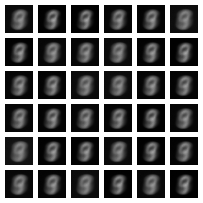
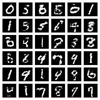
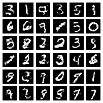
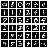
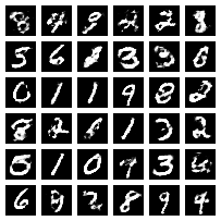
Finally, I’ll share an implementation of WGAN-GP using the MNIST
dataset. Readers can modify it for fun
https://github.com/bojone/gan/
Training progress display:
Original article address: https://kexue.fm/archives/4439
For more details on reprinting, please refer to: Scientific Space FAQ