Now we turn our attention to Riemann curvature. Generally speaking, Riemann curvature provides a scheme that allows someone inside a space to calculate the degree of curvature of the space they inhabit. As the saying goes, “I do not know the true face of Mount Lu, only because I am in the midst of it,” and “The players are confused, while the spectators see clearly.” Therefore, being able to discover the curvature of a space while being within it is a remarkable feat, as if we have transcended our existing space and reached a higher-dimensional space to look down from above. Truly, “As far as the heart can reach, so far the road and the world extend.”
From the perspective of a higher-dimensional space, it is easy to detect the curvature of a space. For example, a geodesic in a curved space appears as a curve when viewed from a higher-dimensional space, allowing for the calculation of curvature and other properties. However, from within the original space, it appears straight; a geodesic is simply the generalization of the concept of a straight line. Therefore, it is impossible to discover the curvature of a space through this direct route; some indirect methods must be employed. These might not be immediately obvious, but once various paths converge to the same result, it feels self-evident.
How can we better derive Riemann curvature so that it clearly reflects the essential difference between curved space and flat space? I have pondered this for a long time and consulted many reference books (Gravitation and Spacetime, Field Theory, Gravitation, etc.), comparing several ways to derive Riemann curvature, which are briefly described below.
The Order of Differentiation Matters
In general tensor analysis or Riemannian geometry textbooks, the way to derive Riemann curvature is by considering the difference in the order of second-order covariant derivatives: A^{\mu}_{;\alpha;\beta}-A^{\mu}_{;\beta;\alpha}=-R^{\mu}_{\nu\alpha\beta}A^{\nu} \tag{40} From this, the Riemann curvature tensor R^{\mu}_{\nu\alpha\beta} can be isolated. This is indeed a straightforward path, but its geometric meaning is not obvious, making it difficult to see how it reflects whether a space is curved or flat. Furthermore, we have not yet defined second-order covariant derivatives (a single covariant derivative results in two indices, making it equivalent to a matrix rather than a vector; defining higher-order covariant derivatives requires attention to detail). Since this definition is essentially pure algebraic calculation and holds little significance for us at the moment, we will not define it here. Readers may refer directly to textbooks, and we will not discuss this scheme further.
Encounter in Curved Space
Additionally, Riemann curvature can be derived through geodesic deviation (which corresponds to tidal forces in general relativity). This is a scheme with clear geometric and physical meaning, but the calculations involved are quite tedious. The main idea is to consider the geodesic equation: \frac{d^2 x^{\mu} }{ds^2}+\Gamma_{\alpha\beta}^{\mu}(x) \frac{d x^{\alpha} }{ds}\frac{d x^{\beta} }{ds}=0 \tag{41} Assuming there is another geodesic x(s)+\delta x(s), it satisfies the equation: \frac{d^2 (x^{\mu} + \delta x^{\mu}) }{ds^2}+\Gamma_{\alpha\beta}^{\mu}(x+\delta x) \frac{d (x^{\alpha}+\delta x^{\alpha}) }{ds}\frac{d (x^{\beta}+\delta x^{\beta}) }{ds}=0 \tag{42} Assuming \delta x and d\delta x/ds are infinitesimal, subtracting the two equations yields: \frac{d^2 \delta x^{\mu}}{ds^2}+\frac{\partial \Gamma_{\alpha\beta}^{\mu}}{\partial x^{\nu}}\delta x^{\nu} \frac{d x^{\alpha} }{ds}\frac{d x^{\beta}}{ds}+2\Gamma_{\alpha\beta}^{\mu}\frac{d \delta x^{\alpha} }{ds}\frac{d x^{\beta}}{ds}=0 \tag{43} Here, \delta x is called the geodesic deviation, and in Riemannian geometry, it is referred to as the “Jacobi vector field.” The above form is already simple enough; however, we prefer to write it in terms of covariant derivatives, as the covariant derivative is the appropriate derivative in curved space. We have previously defined the derivative along a geodesic \frac{DA^{\mu}}{Ds}. By repeating this, we can obtain the second-order derivative along the geodesic \frac{D^2 A^{\mu}}{Ds^2}=\frac{D}{Ds}\left(\frac{DA^{\mu}}{Ds}\right). This is easy to achieve, but since we are not particularly focused on this scheme here, we will not write out the specific form of \frac{D^2 A^{\mu}}{Ds^2}; readers can derive it themselves. After calculation, it is found that: \frac{D^2 \delta x^{\mu}}{Ds^2}=-R^{\mu}_{\nu\alpha\beta}\delta x^{\alpha}\frac{dx^{\nu}}{ds}\frac{dx^{\beta}}{ds} \tag{44} This is where the curvature tensor R^{\mu}_{\nu\alpha\beta} appears. From a mathematical standpoint, a non-zero R^{\mu}_{\nu\alpha\beta} actually indicates an uneven distribution of geodesics, which is one of the manifestations of curved space.
This scheme reminds me of Jimmy Liao’s comic work Turn Left, Turn Right, which tells the story of a male and female protagonist who are used to walking left and right, respectively, so they seemingly never meet. But one day they met at a circular fountain—walking away from each other at one end of the circle and finally meeting at the other end. In curved space, such as on a sphere, even two parallel lines have a chance to intersect. This actually shows that “curvature” is more profound and interesting; it gives our world more possibilities.
Changes After “Strolling” Back
Finally, there is a scheme that analyzes the change in a vector after it is parallel transported along a closed curve. We will analyze this in detail here. In fact, it is equivalent to geodesic deviation, but its geometric meaning is more obvious and helps derive more profound results. It shows that if a vector “strolls” around and returns, it is not necessarily the same as the original vector. The example in the figure below clearly demonstrates this.
Assume there is an arbitrary vector A^{\mu} at x^{\mu}. Starting from x^{\mu}, first transport it by an infinitesimal amount dx^{\mu}, then by an infinitesimal amount \delta x^{\mu}, then by -dx^{\mu}, and finally by -\delta x^{\mu}. That is, it travels around an infinitesimal parallelogram and returns to the origin: x^{\mu}\to x^{\mu}+dx^{\mu}\to x^{\mu}+dx^{\mu}+\delta x^{\mu}\to x^{\mu}+\delta x^{\mu}\to x^{\mu}
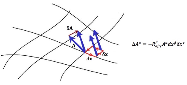
We calculate the change in A^{\mu} step by step during the transport. From x^{\mu} to x^{\mu}+dx^{\mu}, A^{\mu} becomes: A^{\mu}-\Gamma^{\mu}_{\alpha\beta}(x) A^{\alpha}dx^{\beta} \tag{45} Next, from x^{\mu}+dx^{\mu} to x^{\mu}+dx^{\mu}+\delta x^{\mu}, A^{\mu} becomes: \begin{aligned} &A^{\mu}-\Gamma^{\mu}_{\alpha\beta}(x) A^{\alpha}dx^{\beta}-\Gamma^{\mu}_{\nu\gamma}(x+dx) \left[A^{\nu}-\Gamma^{\nu}_{\alpha\beta}(x) A^{\alpha}dx^{\beta}\right]\delta x^{\gamma}\\ =&A^{\mu}-\Gamma^{\mu}_{\alpha\beta}(x) A^{\alpha}dx^{\beta}-\Gamma^{\mu}_{\nu\gamma}(x) A^{\nu} \delta x^{\gamma} \\ &\quad- \frac{\partial \Gamma^{\mu}_{\nu\gamma}(x)}{\partial x^{\beta}} A^{\nu} dx^{\beta} \delta x^{\gamma} + \Gamma^{\mu}_{\nu\gamma}(x) \Gamma^{\nu}_{\alpha\beta}(x) A^{\alpha} dx^{\beta}\delta x^{\gamma} \end{aligned} \tag{46} Here we only keep terms up to the second order.
Similarly, if we consider the change brought by the path x^{\mu}\to x^{\mu}+\delta x^{\mu}\to x^{\mu}+dx^{\mu}+\delta x^{\mu}, we only need to swap dx and \delta x: \begin{aligned} &A^{\mu}-\Gamma^{\mu}_{\alpha\beta}(x) A^{\alpha}\delta x^{\beta}-\Gamma^{\mu}_{\nu\gamma}(x) A^{\nu} d x^{\gamma} \\ &\quad- \frac{\partial \Gamma^{\mu}_{\nu\gamma}(x)}{\partial x^{\beta}} A^{\nu} \delta x^{\beta} d x^{\gamma} + \Gamma^{\mu}_{\nu\gamma}(x) \Gamma^{\nu}_{\alpha\beta}(x) A^{\alpha} \delta x^{\beta} d x^{\gamma} \end{aligned} \tag{47} Naturally, the change caused by the path x^{\mu}+dx^{\mu}+\delta x^{\mu}\to x^{\mu}+\delta x^{\mu}\to x^{\mu} is the negative of the above expression. Thus, the change brought by the entire closed path x^{\mu}\to x^{\mu}+dx^{\mu}\to x^{\mu}+dx^{\mu}+\delta x^{\mu}\to x^{\mu}+\delta x^{\mu}\to x^{\mu} is the difference between the two expressions. Adjusting the summation indices and taking the difference, it is not difficult to obtain: \label{closed_loop_change} \begin{aligned} \Delta A^{\mu} =&-\left(\frac{\partial \Gamma^{\mu}_{\alpha\gamma}}{\partial x^{\beta}}-\frac{\partial \Gamma^{\mu}_{\alpha\beta}}{\partial x^{\gamma}}+\Gamma^{\mu}_{\nu\beta}\Gamma^{\nu}_{\alpha\gamma}-\Gamma^{\mu}_{\nu\gamma}\Gamma^{\nu}_{\alpha\beta}\right)A^{\alpha} dx^{\beta}\delta x^{\gamma}\\ =&-R^{\mu}_{\alpha\beta\gamma} A^{\alpha} dx^{\beta}\delta x^{\gamma} \end{aligned} \tag{48} Here R^{\mu}_{\alpha\beta\gamma}=\frac{\partial \Gamma^{\mu}_{\alpha\gamma}}{\partial x^{\beta}}-\frac{\partial \Gamma^{\mu}_{\alpha\beta}}{\partial x^{\gamma}}+\Gamma^{\mu}_{\nu\beta}\Gamma^{\nu}_{\alpha\gamma}-\Gamma^{\mu}_{\nu\gamma}\Gamma^{\nu}_{\alpha\beta} \tag{49} is the definition of the Riemann curvature tensor; it has 4 indices and is a very “grand” quantity.
In a Nutshell
Three different ways of deriving the Riemann curvature tensor show the difference between curved space and flat space from three perspectives: in flat space, the order of covariant derivatives is interchangeable, while in curved space it is not; in flat space, the distribution of geodesics is uniform and linear, while in curved space it is not; in flat space, a vector does not change after “strolling” around a circle, while in curved space, after “strolling,” it may no longer be the original vector.
Reprinted to please include this article address: https://kexue.fm/archives/4014
For more detailed reprint matters, please refer to: Scientific Space FAQ