Vectors and Connections
Once we establish our own coordinate system at our location, we can perform many measurements. The results of these measurements might be scalars, such as temperature or mass; these quantities remain the same regardless of the coordinate system used. Of course, we sometimes measure vectors, such as velocity, acceleration, or force. These quantities are objective entities, but because the measurement results are expressed in terms of coordinate components, if we change the coordinates, the components will be completely different.
If all locations used the same coordinates, there would naturally be no dispute. However, as we have repeatedly emphasized, people at different locations may use different coordinate systems for various reasons. Therefore, when we write a vector A^{\mu}, strictly speaking, we should also specify that it was measured at position \boldsymbol{x}: A^{\mu}(\boldsymbol{x}). We can only omit this when it does not cause ambiguity.
At this point, we are already able to perform some calculations. For example, if A^{\mu} is measured at \boldsymbol{x}, and the formula for calculating the squared length at \boldsymbol{x} is ds^2 = g_{\mu\nu} dx^{\mu} dx^{\nu}, then the magnitude of A^{\mu} is \sqrt{g_{\mu\nu} A^{\mu}A^{\nu}}, which is an objective entity.
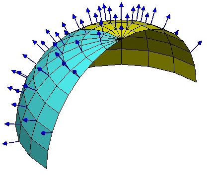
Sometimes we need to compare two vectors at different locations, which involves subtraction. In particular, because the coordinate systems at different locations are different, it is meaningless to directly subtract the components of two vectors from different locations. This is like 5 Chinese Yuan and 5 US Dollars; we cannot conclude that "5 USD - 5 Yuan = (5-5) = 0". However, this situation is only caused by inconsistent unit selection; it would be fine if the same units were chosen. But the measurement of a vector depends not only on the units but also on the coordinate system. For example, when a plane flies from China to the United States, passing through a certain location in China, the measured velocity is (300, 300, 300). When it reaches a certain location in the United States, the measured velocity is also (300, 300, 300), with units in "km/h". However, the measurement in China was done by a Chinese person, and the measurement in the US was done by an American. As everyone knows, the US and China are located on opposite sides of the Earth, and the local coordinate systems they establish are definitely different. Thus, we cannot say that the velocity difference of the plane between the two places is (300-300, 300-300, 300-300) = (0, 0, 0), because it also depends on the direction!
To put it simply, the cause of this problem is that different locations use different coordinate systems—the unit lengths of the coordinates are different, the directions of the coordinate axes are different, and so on. Therefore, we need to transform the vector coordinates from one location into the coordinates of another location before we can compare the components. Here, we only consider the transformation between two positions \boldsymbol{x} and \boldsymbol{x}+d\boldsymbol{x} separated by an infinitesimal distance. That is, how to represent the vector A^{\mu}(\boldsymbol{x}+d\boldsymbol{x}) measured at \boldsymbol{x}+d\boldsymbol{x} (which has its own coordinate system) using the coordinate system at \boldsymbol{x}. Obviously, this involves a transformation matrix, so the key is to determine this transformation matrix.
How do we find this matrix? Imagine that we can place a test vector at \boldsymbol{x}, then move this vector to \boldsymbol{x}+d\boldsymbol{x} and see what it becomes. As long as there are enough test vectors, we can determine this transformation matrix. Therefore, we need a set of the most natural test vectors to provide us with a reference. We already know that the geodesic is an objective entity; in fact, the geodesic provides the most natural reference, nothing is more natural than it. We can rewrite the geodesic equation as: d\left(\frac{d x^{\mu} }{ds}\right)=-\Gamma_{\alpha\beta}^{\mu} \frac{d x^{\alpha} }{ds}d x^{\beta} \tag{28} This formula means that if there is a unit vector \frac{dx^{\mu}}{ds} at the current position \boldsymbol{x}, then after moving forward by d\boldsymbol{x} along the geodesic direction, the change in the unit vector \frac{dx^{\mu}}{ds} is d\left(\frac{d x^{\mu} }{ds}\right), which is also equal to -\Gamma_{\alpha\beta}^{\mu} \frac{d x^{\alpha} }{ds}d x^{\beta}, i.e., \frac{dx^{\mu}}{ds}\quad\to\quad \frac{dx^{\mu}}{ds}-\Gamma_{\alpha\beta}^{\mu} \frac{d x^{\alpha} }{ds}d x^{\beta} \tag{29} Then, the coordinate transformation matrix (Jacobian matrix) from \boldsymbol{x} to \boldsymbol{x}+d\boldsymbol{x} is: \frac{\partial\left(\frac{dx^{\mu}}{ds}-\Gamma_{\alpha\beta}^{\mu} \frac{d x^{\alpha} }{ds}d x^{\beta}\right)}{\partial \frac{dx^{\nu}}{ds}}=\delta_{\nu}^{\mu}-\Gamma_{\nu\beta}^{\mu} d x^{\beta} \tag{30} Conversely, the coordinate transformation matrix from \boldsymbol{x}+d\boldsymbol{x} to \boldsymbol{x} is: \label{lianluo}\delta_{\nu}^{\mu}+\Gamma_{\nu\beta}^{\mu} d x^{\beta} \tag{31} Viewed this way, the coefficients \Gamma_{\alpha\beta}^{\mu} connect the coordinates at \boldsymbol{x} and \boldsymbol{x}+d\boldsymbol{x}, so it is very appropriate to call them “connection coefficients”.
Knowing the coordinate transformation method, it is easy to see that if we place A^{\mu}(\boldsymbol{x}+d\boldsymbol{x}) at position \boldsymbol{x} for measurement, the result will be: \left(\delta_{\nu}^{\mu}+\Gamma_{\nu\beta}^{\mu} d x^{\beta}\right) A^{\nu}(\boldsymbol{x}+d\boldsymbol{x})=A^{\mu}(\boldsymbol{x}+d\boldsymbol{x})+\Gamma_{\nu\beta}^{\mu} A^{\nu}(\boldsymbol{x}+d\boldsymbol{x}) d x^{\beta} \tag{32}
Covariant Derivative
We previously mentioned the need to subtract vectors, and in the section on connections, we studied the coordinate transformation between two positions separated by an infinitesimal distance, obtaining the result of equation (32): if A^{\mu}(\boldsymbol{x}+d\boldsymbol{x}) is measured at position \boldsymbol{x}, the result is: A^{\mu}(\boldsymbol{x}+d\boldsymbol{x})+\Gamma_{\nu\beta}^{\mu} A^{\nu}(\boldsymbol{x}+d\boldsymbol{x}) d x^{\beta} \tag{33} In this way, we can directly perform subtraction because the two vectors are now measured at the same location: A^{\mu}(\boldsymbol{x}+d\boldsymbol{x})+\Gamma_{\nu\beta}^{\mu} A^{\nu}(\boldsymbol{x}+d\boldsymbol{x}) d x^{\beta}-A^{\mu}(\boldsymbol{x}) \tag{34} We can study the limiting case: \lim_{d\boldsymbol{x} \to 0} \frac{A^{\mu}(\boldsymbol{x}+d\boldsymbol{x})+\Gamma_{\nu\beta}^{\mu} A^{\nu}(\boldsymbol{x}+d\boldsymbol{x}) d x^{\beta}-A^{\mu}(\boldsymbol{x})}{dx^{\beta}} \tag{35} It is not difficult to see that the result will be: \frac{\partial A^{\mu}}{\partial x^{\beta}}+\Gamma_{\nu\beta}^{\mu} A^{\nu} \tag{36} This is called the covariant derivative of the vector A^{\mu}, denoted as: A^{\mu}_{;\beta}=\frac{\partial A^{\mu}}{\partial x^{\beta}}+\Gamma_{\nu\beta}^{\mu} A^{\nu} \tag{37} Naturally, the following result is called the covariant differential: D A^{\mu}=dA^{\mu}+\Gamma_{\nu\beta}^{\mu} A^{\nu}dx^{\beta} \tag{38} If divided by the line element ds, we obtain the derivative: \frac{D A^{\mu}}{Ds}=\frac{dA^{\mu}}{ds}+\Gamma_{\nu\beta}^{\mu} A^{\nu}\frac{dx^{\beta}}{ds} \tag{39} It can be seen that the result depends on the choice of the curve x^{\beta}. We generally choose it to be a geodesic, and the above expression is called the geodesic derivative (derivative along a geodesic).
Reviewing the entire process, our starting point for deriving the covariant derivative is: Directly subtracting vector components from two different locations is meaningless. If necessary, one must transform a vector from one location to another. Studying the limit case yields the covariant derivative. The covariant derivative is a definition of a derivative with geometric meaning in space, and thus it is also an objective entity.
In general tensor analysis or Riemannian geometry textbooks, there are many ways to derive the covariant derivative. Some textbooks adopt this approach: Because we know the specific form of the gradient in Cartesian coordinates, we start from the Cartesian coordinate system and obtain the derivative forms in other coordinate systems through transformation laws. This seems reasonable, but it actually implies an assumption of flat space—that is, although curvilinear coordinates are used, they can be transformed back to Cartesian coordinates through some transformation; otherwise, this approach is invalid. This means the space is flat; the fact that curved spaces yield the same result is, in a sense, just a coincidence. If the same logic is used to derive the Riemann curvature, the result will be identically zero—because the space was flat to begin with.
There are other derivation methods as well. Overall, I believe most methods are “not geometric enough” and are more about algebraic manipulation. The author here has used a more geometric approach.
Please include the address of this article when reprinting: https://kexue.fm/archives/3998
For more detailed reprinting matters, please refer to: Scientific Space FAQ