As the first step of an OCR system, feature extraction aims to identify candidate text region features in an image, facilitating text localization in the second step and recognition in the third. In this section, we focus on mimicking the human eye’s process of handling images and Chinese characters, taking an innovative path in image processing and character localization. This part of the work is the core of the entire OCR system and the most central part of our research.
Traditional text segmentation approaches mostly follow the logic of "edge detection + erosion/dilation + connected component detection," as seen in literature [1]. However, performing edge detection on images with complex backgrounds leads to excessive edges in background areas (i.e., increased noise), while edge information in text areas is easily ignored, resulting in poor performance. If erosion or dilation is performed at this stage, the background regions will merge with the text regions, further worsening the results. (In fact, we have traveled far enough down this path; we even wrote our own edge detection functions for this purpose. After extensive testing, we ultimately decided to abandon this approach.)
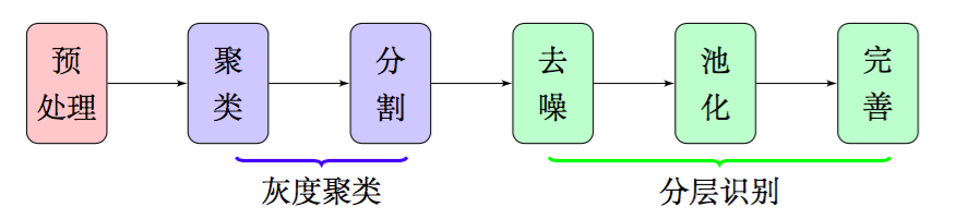
Therefore, in this article, we abandon edge detection and erosion/dilation. Through steps such as clustering, segmentation, denoising, and pooling, we obtain high-quality features of the text portions. The overall process is roughly shown in Figure 2. These features can even be directly input into a text recognition model for identification without additional processing. Since each part of our results is supported by a corresponding theoretical foundation, the reliability of the model is guaranteed.
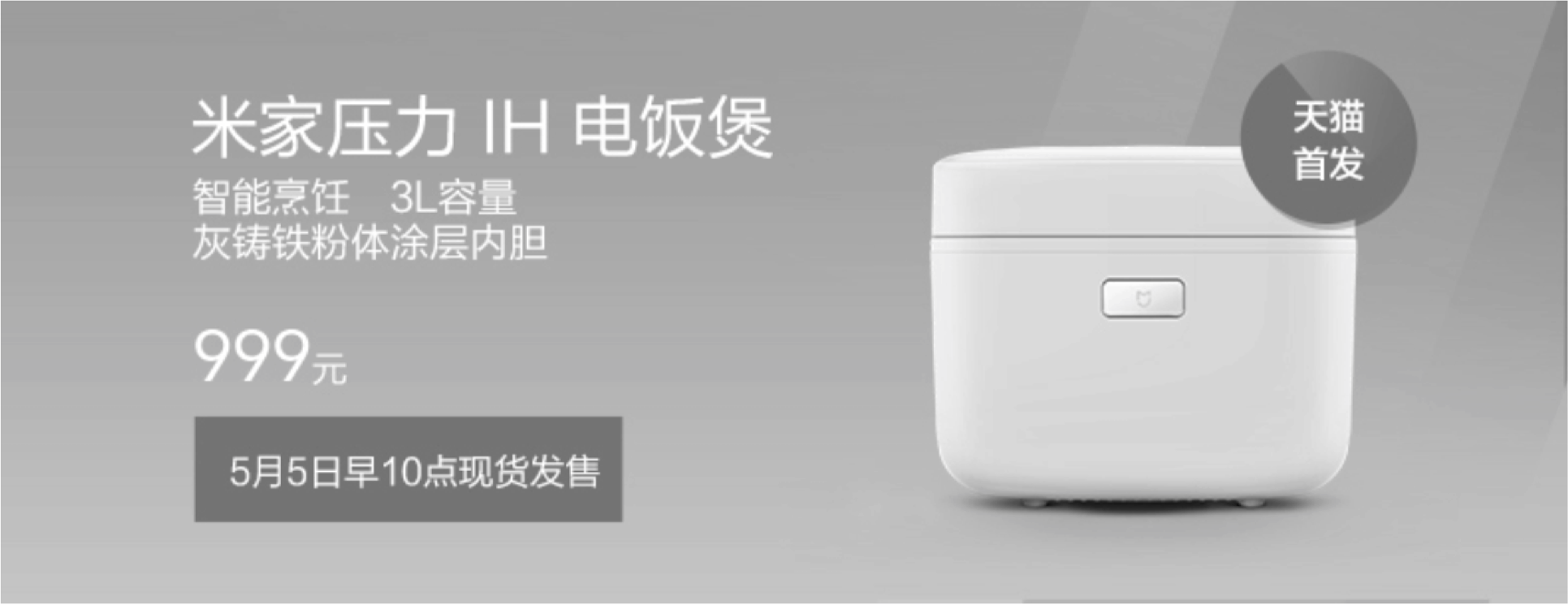
In this part of the experiment, we use Figure 3 to demonstrate our results. The characteristics of this image are its medium size, dazzling background, rich colors, and a mixed layout of text and images with no fixed format—a typical e-commerce promotional image. As can be seen, the key to processing this image is how to distinguish between image regions and text regions, identifying and removing the electric rice cooker on the right while retaining only the text areas.

Image Preprocessing
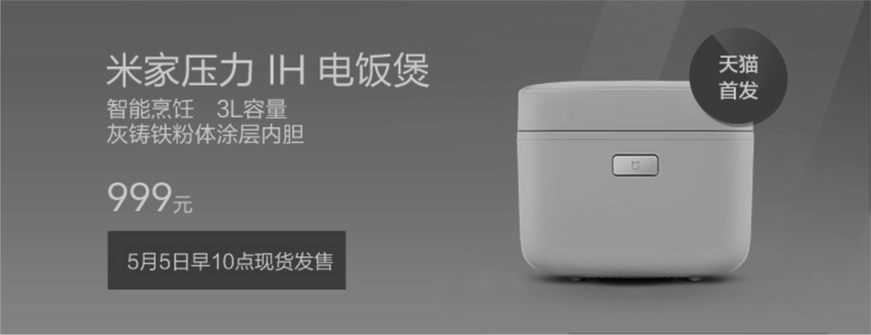
First, we read the original image as a grayscale image to obtain an m \times n grayscale matrix M, where m and n are the height and width of the image. Reading the image this way results in lower dimensionality than a direct RGB color image without significant loss of text information. Converting to a grayscale image essentially integrates the three channels of the original RGB image into a single channel using the following formula: Y = 0.299R + 0.587G + 0.114B \tag{1} The grayscale version of Figure 3 is shown below.
The dimensions of the image itself are not large. If processed directly, the strokes of the characters might be too small and easily treated as noise. Therefore, to ensure the strokes have a certain thickness, the image can be enlarged first. In our experiments, enlarging the image to twice its original size generally yields good results.
However, after enlargement, the distinction between text and background decreases. This is because interpolation algorithms are used to fill in missing pixels during enlargement. At this point, it is necessary to increase the contrast accordingly. After testing, a "power transformation" with an exponent of 2 works well for most images. The power transformation is: x \mapsto x^r \tag{2} where x represents an element in matrix M, and r is the exponent, which we choose as 2. Then, the results need to be mapped to the [0, 255] range: x \mapsto \frac{x - M_{min}}{M_{max} - M_{min}} \times 255 \tag{3} where M_{max} and M_{min} are the maximum and minimum values of matrix M. After this processing, the image appears as follows:
Grayscale Clustering
Next, we cluster the colors of the image. There are two factual bases for clustering:
1. Grayscale Resolution: The human eye’s grayscale resolution is approximately 40; therefore, pixel values like 254 and 255 both appear as white to us.
2. Design Principles: According to general aesthetic principles, when considering poster design or clothing coordination, it is usually required that the color combination does not exceed three colors.
More colloquially, although the grayscale range of an image is [0, 255], the overall tones we perceive are generally few. Therefore, similar grayscale levels can be grouped into one category, thereby reducing the color distribution and effectively lowering noise.
In fact, clustering is a process of adaptively performing multi-thresholding based on image characteristics, avoiding the information loss caused by traditional simple binarization. Since we need to automatically determine the number of clusters, traditional clustering methods like K-Means were discarded. Furthermore, our tests showed that feasible clustering methods like MeanShift suffer from defects such as slow speed. Consequently, we designed our own clustering method using a "Kernel Density Estimation" approach, clustering by finding the local maxima of color density.
Kernel Density Estimation
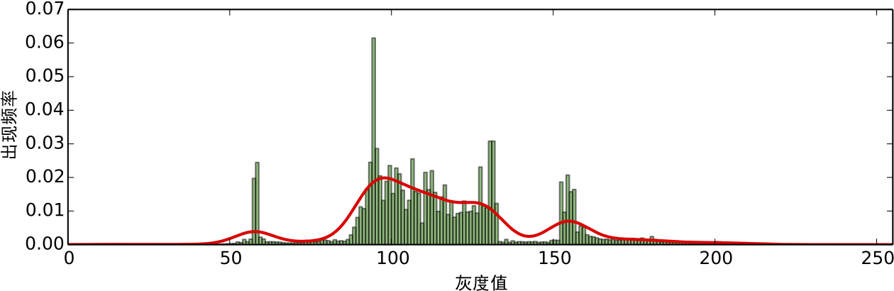
After preprocessing the image, we can count the occurrences of each grayscale level to obtain a frequency distribution histogram as shown in Figure 5:

It can be seen that the distribution of grayscale levels forms several prominent peaks; in other words, there is a certain clustering trend. However, the statistical results of a histogram are discrete. A smooth result is more convenient for analysis and research, and the results are more convincing. The method to smooth statistical results is Kernel Density Estimation (KDE).
KDE is a non-parametric estimation method proposed by Rosenblatt and Parzen, which is highly regarded in statistical theory and applications [2]. Of course, it can also be simply viewed as a function smoothing method. When we estimate the probability (density) of a certain value appearing based on a large amount of data, we are essentially performing the following calculation: \hat{p}(x) = \frac{1}{nh} \sum_{i=1}^n K\left(\frac{x - x_i}{h}\right) \tag{4} where K(x) is called the kernel function. When h is set to 1 and K(x) is chosen as: K(x) = \left\{\begin{aligned}&1, \, x=0\\ &0, \, x \neq 0\end{aligned}\right. \tag{5} it results in the histogram estimation mentioned above. The term K(x) is simple: it tells us that all x_i within the range h are counted towards x, and how they are counted is given by K(\frac{x - x_i}{h}). Clearly, the choice of h significantly affects the result; h is called the bandwidth, and it primarily affects the smoothness of the result.
If K(x) is discrete, the result remains discrete, but if K(x) is smooth, the result will also be relatively smooth. A commonly used smooth kernel is the Gaussian kernel: K(x) = \frac{1}{\sqrt{2\pi}} e^{-x^2/2} \tag{6} The resulting estimate is also called Gaussian Kernel Density Estimation. Here, we use Scott’s rule to adaptively select h, but a smoothing factor must be manually specified; in this article, we select 0.2. For the example image, we obtain the red curve result shown in Figure 6.
Maxima and Minima Segmentation
From Figure 6, we can further see that the image indeed exhibits a clustering trend. This is manifested by several obvious local maxima and minima. The maxima are located at x = 10, 57, 97, 123, 154, and the minima are at 25, 71, 121, 142.
Therefore, a very natural clustering method is: cluster into as many categories as there are local maxima, using the local minima as the boundaries between categories. That is to say, for Figure 3, the image can be divided into 5 layers and processed layer by layer. After layering, the shape of each layer is as follows, where white is 1 and black is 0.

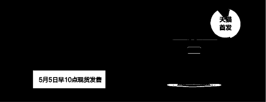
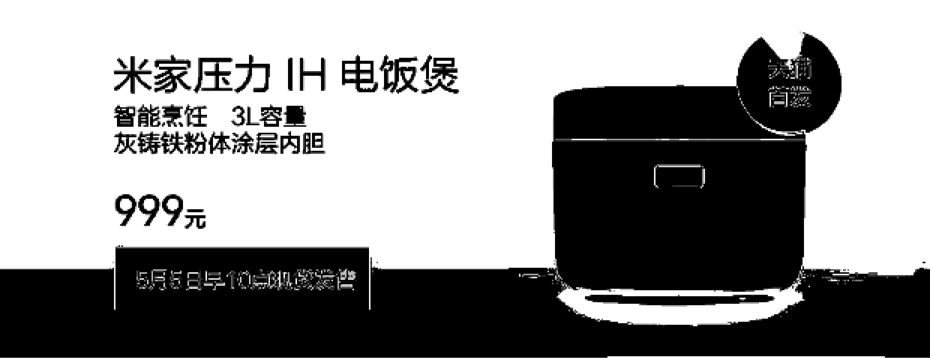

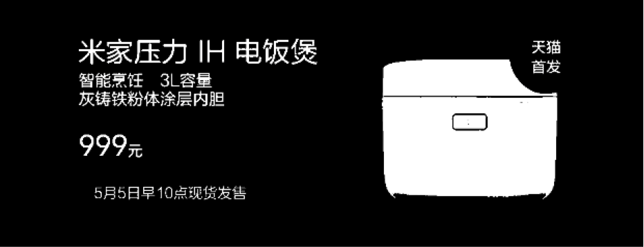
The image is divided into 5 layers through clustering
Evidently, due to the "contrast" and "gradient" assumptions, text layers can indeed be separated using the KDE-based clustering method. Moreover, by using the clustering-layering approach, there is no need to make any assumptions about the text color; even when the text color is identical to the background color, effective detection can still be achieved.
Original article address: https://kexue.fm/archives/3785
For more details on reposting, please refer to: Scientific Space FAQ