Review of the Previous Part
In the first part, we introduced the concept of “entropy” and its origins. The formula for entropy is: S = -\sum_x p(x) \log p(x) \tag{1} or S = -\int p(x) \log p(x) dx \tag{2} In the first part, we learned that entropy represents both uncertainty and information content; in fact, they are the same concept.
Having discussed the concept of entropy, we now move on to the “Maximum Entropy Principle.” The Maximum Entropy Principle tells us that: When we want to obtain the probability distribution of a random event, if there is not enough information to completely determine this distribution (perhaps the type of distribution is unknown, or the type is known but several parameters are undetermined), the most “safe” approach is to choose the distribution that maximizes entropy.
The Maximum Entropy Principle
Admitting Our Ignorance
Many articles, when introducing the Maximum Entropy Principle, cite the famous saying—“Don’t put all your eggs in one basket”—to explain the principle in layman’s terms. However, I personally believe this phrase misses the mark and does not well-reflect the essence of the Maximum Entropy Principle. I believe a more appropriate explanation is: Admitting our ignorance!
How should we understand the connection between this phrase and the Maximum Entropy Principle? We already know that entropy is a measure of uncertainty. Maximum entropy implies maximum uncertainty. Therefore, choosing the distribution with the maximum entropy means we are choosing the distribution for which we are most ignorant. In other words, admit our ignorance about the problem and do not deceive ourselves. We might be able to deceive each other, but we can never deceive Nature.
For example, when flipping a coin, we generally assume the probability of heads and tails is the same. At this point, entropy is maximized, and we are in a state of maximum ignorance regarding the coin. If someone were very confident that the probability of heads is 60% and tails is 40%, they must know that the coin has been tampered with to make heads more likely. Thus, that person’s level of understanding of the coin is higher than ours. If we do not have access to that information, we should honestly admit our ignorance and assume the probabilities are equal, rather than making subjective conjectures (because there are too many things one could subjectively guess; if we wrongly assumed the probability of tails was higher, it would lead to even greater losses).
Therefore, selecting the model with maximum entropy signifies our honesty towards Nature. We believe that if we are honest with Nature, Nature will not treat us poorly. This is the philosophical significance of the Maximum Entropy Principle. Furthermore, admitting our ignorance means we assume we can obtain the maximum amount of information from it, which, in a sense, also conforms to the principle of maximum economy.
Estimating Probabilities
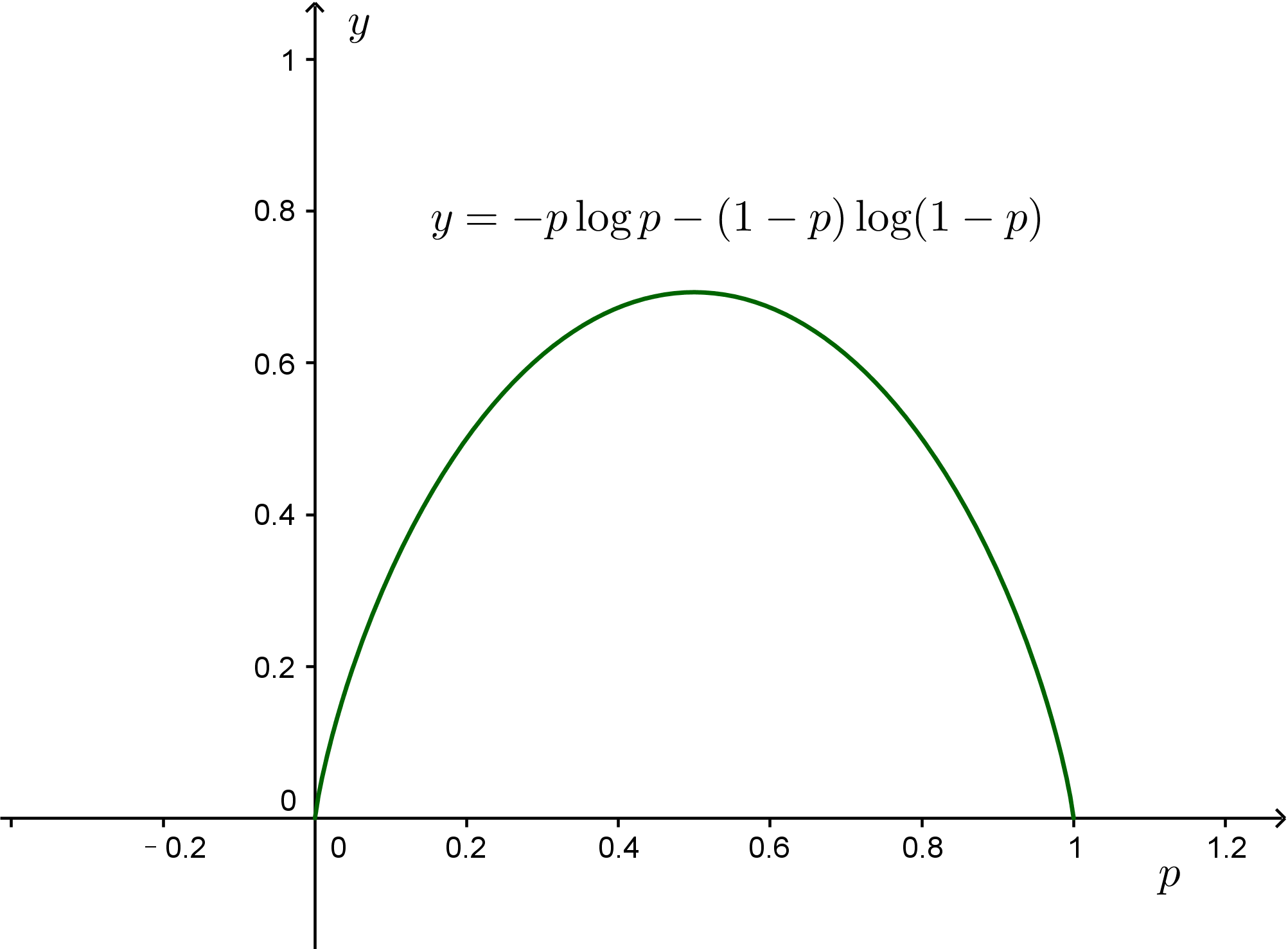
Having said so much, we haven’t actually calculated anything yet, and words alone are hardly persuasive. First, let’s solve the simplest problem: using the Maximum Entropy Principle to explain why we believe the probability of both sides is \frac{1}{2} when flipping a coin. Suppose the probability of heads is p; then the entropy is: S(p) = -p \log p - (1-p) \log (1-p) \tag{15} By taking the derivative, we find that S(p) is maximized when p=\frac{1}{2}. Thus, we guess the probability of each side is \frac{1}{2}. Similarly, it can be proven using the Maximum Entropy Principle that when rolling a die, the probability of each face should be \frac{1}{6} (this is a multivariable calculus problem). If there are n possibilities, the probability of each should be \frac{1}{n}.
Note that the above estimates are made under the assumption of complete ignorance. In fact, we are often not that ignorant. We can derive some information from a large amount of statistics to refine our understanding. Consider the following example:
A fast-food restaurant offers 3 types of food: Burger (1), Chicken (2), and Fish (3). The prices are 1 Yuan, 2 Yuan, and 3 Yuan, respectively. It is known that the average expenditure of customers in this shop is 1.75 Yuan. Find the probability of customers purchasing these 3 types of food.
Here, “the average expenditure of customers in this shop is 1.75 Yuan” is a result we obtained from extensive statistics. If we assumed complete ignorance, we would get a probability of \frac{1}{3} for each food item, but then the average expenditure would be 2 Yuan, which does not match the fact. In other words, we are not completely ignorant about the purchasing situation; we at least know the average expenditure is 1.75 Yuan. This fact helps us estimate the probabilities more accurately.
Estimation Framework
Discrete Probabilities
These “facts” that help us estimate probabilities more accurately might be our life experiences or some prior information. Regardless, they must be statistical results. The mathematical description is given as constraints in the form of expectations: E[f(x)] = \sum_{x} p(x)f(x) = \tau \tag{16} Note that although we are no longer completely ignorant, we must still admit our ignorance—an ignorance maintained under the premise of knowing certain facts. Mathematically, the problem becomes finding the maximum of equation (1) under k constraints of the form (16). For the fast-food example, f(x)=x, so: \sum_{x=1,2,3} p(x)x = 1.75 \tag{17} We seek to maximize -\sum_x p(x) \log p(x). This type of problem is a constrained extremum problem in calculus, and the method to solve it is the Lagrange Multiplier Method. By introducing parameters \lambda, the original problem is equivalent to finding the extremum of: -\sum_x p(x) \log p(x) - \lambda_0 \left(\sum_x p(x) - 1\right) - \lambda_1 \left(\sum_x p(x)x - 1.75\right) \tag{18} In equation (18), we introduced two constraints: the first is universal (the sum of all p(x) is 1), and the second is the “fact” we recognized. Solving the derivatives yields the extremum at p(1) = 0.466, p(2) = 0.318, p(3) = 0.216, where entropy is maximized.
More generally, if there are k constraints, we must find the extremum of: \begin{aligned} -\sum_x p(x) \log p(x) & - \lambda_0 \left(\sum_x p(x) - 1\right) - \lambda_1 \left(\sum_x p(x)f_1(x) - \tau_1\right) \\ & - \dots - \lambda_k \left(\sum_x p(x)f_k(x) - \tau_k\right) \end{aligned} \tag{19} Equation (19) is easily solved to give: p(x) = \frac{1}{Z} \exp \left( -\sum_{i=1}^k \lambda_i f_i(x) \right) \tag{20} where Z is the normalization factor: Z = \sum_x \exp \left( -\sum_{i=1}^k \lambda_i f_i(x) \right) \tag{21} Substituting equation (20) into: \sum_x p(x)f_i(x) - \tau_i = 0, \quad (i=1, 2, \dots, k) \tag{22} allows us to solve for the unknown \lambda_i. (Unfortunately, for general f_i(x), the above equation has no simple solution, and even numerical solutions are difficult, which makes maximum entropy models relatively hard to use.)
Continuous Probabilities
Note that equations (19), (20), (21), and (22) are derived for discrete probabilities. The results for continuous probabilities are similar. Equation (19) corresponds to: \begin{aligned} -\int p(x) \log p(x) dx & - \lambda_0 \left(\int p(x) dx - 1\right) - \lambda_1 \left(\int p(x)f_1(x) dx - \tau_1\right) \\ & - \dots - \lambda_k \left(\int p(x)f_k(x) dx - \tau_k\right) \end{aligned} \tag{23} Finding the maximum of (23) is actually a problem in the calculus of variations. However, since no derivative terms appear, this variational problem is not much different from ordinary differentiation. The result is still: p(x) = \frac{1}{Z} \exp \left( -\sum_{i=1}^k \lambda_i f_i(x) \right) \tag{24} where Z = \int \exp \left( -\sum_{i=1}^k \lambda_i f_i(x) \right) dx \tag{25} Similarly, we substitute (24) into: \int p(x)f_i(x) dx - \tau_i = 0, \quad (i=1, 2, \dots, k) \tag{26} to solve for the parameters \lambda_i.
Examples of Continuous Cases
Solving continuous cases is sometimes easier. For example, if there is only one constraint f(x)=x (knowing the mean of the variable), the probability distribution is an exponential distribution: p(x) = \frac{1}{Z} \exp(-\lambda x) \tag{27} The normalization factor is: \int_0^{\infty} \exp(-\lambda x) dx = \frac{1}{\lambda} \tag{28} So the probability distribution is: p(x) = \lambda \exp(-\lambda x) \tag{29} The constraint is: \tau = \int_0^{\infty} \lambda \exp(-\lambda x) x dx = \frac{1}{\lambda} \tag{30} Thus the result is: p(x) = \frac{1}{\tau} \exp\left(-\frac{x}{\tau}\right) \tag{31}
Furthermore, if there are two constraints, f_1(x)=x and f_2(x)=x^2 (equivalent to knowing the mean and variance), the probability distribution is the Normal Distribution (note, the normal distribution appears again): p(x) = \frac{1}{Z} \exp(-\lambda_1 x - \lambda_2 x^2) \tag{32} The normalization factor is: \int_{-\infty}^{\infty} \exp(-\lambda_1 x - \lambda_2 x^2) dx = \sqrt{\frac{\pi}{\lambda_2}} \exp\left(\frac{\lambda_1^2}{4\lambda_2}\right) \tag{33} So the probability distribution is: p(x) = \sqrt{\frac{\lambda_2}{\pi}} \exp\left(-\frac{\lambda_1^2}{4\lambda_2}\right) \exp(-\lambda_1 x - \lambda_2 x^2) \tag{34} The two constraints are: \begin{aligned} & \tau_1 = \int_{-\infty}^{\infty} \sqrt{\frac{\lambda_2}{\pi}} \exp\left(-\frac{\lambda_1^2}{4\lambda_2}\right) \exp(-\lambda_1 x - \lambda_2 x^2) x dx = -\frac{\lambda_1}{2\lambda_2} \\ & \tau_2 = \int_{-\infty}^{\infty} \sqrt{\frac{\lambda_2}{\pi}} \exp\left(-\frac{\lambda_1^2}{4\lambda_2}\right) \exp(-\lambda_1 x - \lambda_2 x^2) x^2 dx = \frac{\lambda_1^2 + 2\lambda_2}{4\lambda_2^2} \end{aligned} \tag{35} Substituting the solved results into (34) yields: p(x) = \sqrt{\frac{1}{2\pi(\tau_2 - \tau_1^2)}} \exp\left( -\frac{(x - \tau_1)^2}{2(\tau_2 - \tau_1^2)} \right) \tag{36} Note that \tau_2 - \tau_1^2 is exactly the variance. Therefore, the result is exactly a normal distribution with mean \tau_1 and variance \tau_2 - \tau_1^2!! This serves as another origin for the normal distribution!
When reprinting, please include the original address of this article: https://kexue.fm/archives/3552
For more detailed reprinting matters, please refer to: Scientific Space FAQ